Abstract
We used discrete-choice experiments (DCE) to elicit farmers’ preferences among alternative agri-environmental schemes (AES) designed to reduce soil risk of erosion, maintain soil fertility, enhance countryside landscape, and preserve agrobiodiversity in arable lands of Sicily (Italy). Using appropriate models, we also investigated farmers’ preference heterogeneity and spatial correlation. The results demonstrated a general positive and highly heterogeneous attitude in farmers toward the adoption of environmentally friendly practices and suggested the need of modulate AES according to preferences’ heterogeneity respect to sustainable agricultural practices and local contexts.
DOI: 10.30682/nm1804e
Maria De Salvo*, Giuseppe Cucuzza*, Salvatore Luciano Cosentino*,
Lea Nicita*, Giovanni Signorello*
* Department of Agriculture, Food and Environment (Di3A), University of Catania, Italy.
Corresponding author: mdesalvo@unict.it.
1. Introduction
Agri-environmental schemes (AES) represent the principal policy instruments to enhance agricultural sustainability (McWilliam, 2017). Through AES, farmers are encouraged to protect the environment on their farmland in exchange for per-hectare compensation calculated using a “supply-side” prospective (Muradian et al., 2010).
The approach generally adopted by policymakers to design AES presents some weaknesses that may limit either the effectiveness or the efficiency of AES as sustainability tool. Compensations are often established on the basis of income forgone and/or additional costs associated with the adoption of more sustainable practices. The premium for the risk associated with the adoption of a conservation plan is generally not considered (Cooper and Signorello, 2008). The common method of establishing economic compensation and the “fixed” nature of this compensation do not consider spatial variability of costs and benefits associated with eco-friendly practices and exclude the possibility of further compensation for farmers who are willing to practice high-level environmental management (Mullan and Kontoleon, 2012; Whittington and Pagiola, 2012). Moreover, heterogeneity of preferences is often not considered in AES design, despite numerous studies demonstrating the presence of large variation in AES preferences among farmers and spatial context (Matta et al., 2009; Ruto and Garrod, 2009; Espinosa-Goded et al., 2010; Christensen et al., 2011; Broch and Vedel, 2012).
Previous research on the determinants of farmers’ participation in AES is principally based on actual participation behavior (Defrancesco et al., 2008; Hynes and Garvey, 2009), rather than on contingent behavior.
Information on how farmers percept such schemes and how react when their characteristics are modified in hypothetical scenarios could provide important inputs to better design AES and increase the farmers’ participation rate (Espinosa-Goded et al., 2010). Contingent behavior experiments could inform policymakers about heterogeneity in relation to AES content. Given that both the costs and the benefits associated with sustainable practices are also subject to spatial variation, the need of spatially designed AES emerges (Wätzold and Drechsler, 2005). Improving the spatial targeting of policy tools could improve their cost-effectiveness and support better policy design solutions (Vergamini et al., 2013).
To address these research requirements, we implement a stated-preference study that simulates the steps that should precede the definition of agri-environmental contracts. The objective of this study is twofold. First, we analyze farmers’ preferences for alternative AES schemes, highlighting which sustainable goals are perceived as more important, and evidencing farmers’ willingness to adopt proposed schemes. Second, we explore farmers’ preference heterogeneity and detect the presence of “neighborhood effects” to assess the role of spatial correlation in farmers’ preferences. The case study concerns grain growers in inland areas of Sicily. Farmers’ preferences are elicited through a discrete-choice experiments (DCE) exercise.
2. Related empirical literature
Stated preference methods (Bateman et al., 2002), such as Contingent Valuation Method (CVM) and DCE, have been extensively used to estimate compensation for farmers adopting contracts devoted to enhancing agricultural sustainability. Cooper and Signorello (2008), Dupraz et al. (2003), and Nyongesa et al. (2016) are only a few examples of CVM applications. However, to investigate preferences for alternative AES, the DCE approach seems more appropriate because it allows greater possibility of better understanding the preferences related to the supply of ecosystem services (Campbell et al., 2009; Vedel et al., 2010). A great deal of studies (Ruto and Garrod, 2009; Espinosa-Goded et al., 2010; Christensen et al., 2011; Broch and Vedel, 2012; Costedoat et al., 2016; Greiner et al., 2014; and Vorlaufer et al., 2017; Randrianarison et al., 2017) have demonstrated that farmers’ choice of AES schemes does not depend on the commitments of production practices, but rather depends heavily on contract peculiarities. Previous research has also designed DCE on the level of farmers’ commitments to achieving sustainability goals. For example, Espinosa-Goded et al. (2010) investigate farmers’ agri-environmental preferences for contracts that vary depending on the amount of land to be enrolled in the AES, the availability of compulsory and free-of-charge technical training and advisory services, and economic compensation. Jaeck and Lifran (2009) study the sensitivity of farmers to payment for agri-environmental services in the context of strong ecological and policy constraints. Shultz et al. (2014) explore farmers’ prospective responses to the “greening” of common agricultural policy (CAP), comparing an “opt-out” alternative with a “greening” alternative. Other AES studies focus on the protection of biodiversity in natural regions (Greiner et al., 2014), in home gardens (Birol et al., 2006; Birol et al., 2009), in forests (Matta et al., 2009; Santos et al., 2015; Lienhoop et al., 2015; Vorlaufer et al., 2017; Felardo and Berrens, 2018) and in arable land (Vaissière et al., 2017). Other EAS studies address soil conservation (Tesfaye et al., 2014), water-related ecosystem services (Beharry-Borg and Scarpa, 2010; Mulatu et al., 2014; Chaikaew et al., 2017) pesticide-free buffer zones (Christensen et al., 2011), optimization of fertilizer use (Wuepper et al., 2017), agriculture in protected and buffer areas (Rocchi et al., 2017), olive grove subsystems (Villanueva et al., 2017) silvopastoral systems (Raes et al., 2017), climate regulating services in agricultural systems (Aslam et al., 2017) and flood control (Zandersen et al., 2016).
Wätzold and Drechsler (2005), Drechsler et al. (2007), and Bamière et al. (2011) evidence the importance of spatial patterns in designing AES.
3. Materials and method
3.1. Experimental design
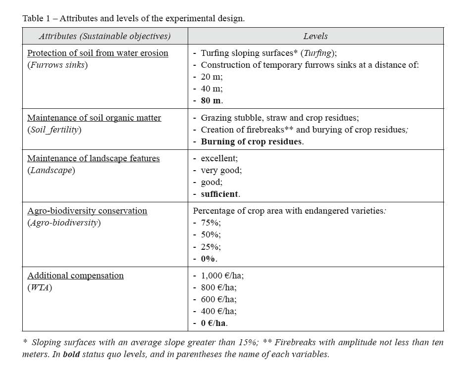
In this study, we designed a DCE where farmers have the possibility to choose among hypothetical AES, that are more binding than the current local regulatory framework. The simulated scenarios were modulated on five attributes. Four attributes were concerned with agricultural sustainability goals. The fifth attribute was the additional cash compensation that farmers could receive for their participation in a more coercive AES.
Attributes used to identify agri-environmental objectives in each AES were the following: 1) the protection from erosion of sloping terrain; 2) the maintenance of soil organic matter; 3) the maintenance of countryside landscape features; 4) the conservation of agrobiodiversity. To reduce the risk of erosion in sloping terrain (e.g., with an average slope greater than 15%), we proposed the following agricultural practices: 1) the construction of temporary sink furrows with an inter-distance equal to 20 m, 40 m or 80 m (minimum level); 2) the permanent cover of these surfaces with grassy or crops for the entire crop year. To conserve the soil’s organic matter, we relied on proper management of stubble and plant residues. The minimum level of intervention concerned the burning of stubble, straw, and crop residues when the risk of fire is lower. More sustainable practices included the following actions: 1) perimeter firebreaks (with amplitude not less than 10 meters) to prevent the spread of fire from adjacent fields and proceed with the burial of crop residues; 2) grazing the entire surface affected by stubble, straw, and crop residues. For the maintenance of landscape features (e.g., terraces, ban trees, groves, and water mirrors), we considered the effort of a farmer to maintain landscape features from a sufficient level of maintenance (minimum level) to an excellent level of maintenance. In relation to the goal of agrobiodiversity conservation, we ask farmers to cultivate local endangered varieties. This attribute varied from zero (minimum level) to 75% of the total crop area. Each hypothetical AES scheme implied an increase in the level of the ecosystem services provided by farmers in relation to the levels required by the local current regulations. To compensate farmers for greater effort, an additional monetary compensation to the currently received economic support was offered. This compensation ranged between 400 €/ha and 1,000 €/ha, and represents an “environmental premium” that compensates farmers either for the higher opportunity cost/income forgone or for the risk associated with the adoption of a sustainable plan that is stricter.
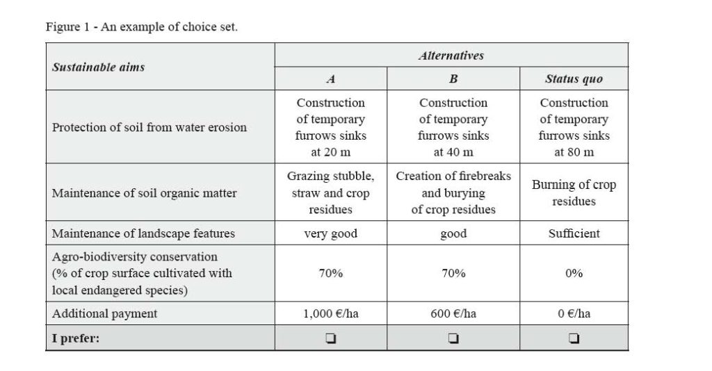
Attributes and levels employed to create alternative scenarios are reported in Table 1. The corresponding full factorial design lead to 288 alternative scenarios (alternatives). Given that this number was too large if compared with operating constraints, we implemented an orthogonal main-effect-only design, which reduced the number alternative profiles to sixteen. Each of these alternatives represents option A in the choice set. Option B is identified by the fold-over technique (Hensher et al., 2015). The status quo was identified as the minimum level for each attribute. An example of the choice set is presented in Figure 1. Farmers were asked to select among the option A, option B and the status quo, in an iterative manner, four times.
The final questionnaire was designed on the basis of the results obtained through focus groups and pilot surveys. It includes a series of questions aimed at: 1) identifying the technical and agronomic farm peculiarities; 2) detecting the cultivation techniques and methods (crop rotation, species and varieties used, type of work performed, fertilization and weed control); 3) gathering farmers’ (respondents’) socio-economics profiles and attitudes concerning maintenance of soil fertility, reduction the risk of erosion, protection of agricultural landscape and conservation of agrobiodiversity.
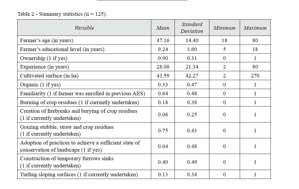
The interviews covered a random sample of 125 cereal farmers who grow crops in the Sicilian slopes inland areas, with average gradients of farmland over 15%. Table 2 reports the summary statistics of the sample.
3.2. Econometric models
To analyse DCE data we used econometric models based on random utility maximization framework (McFadden, 2001). The utility (Uni) of i-th alternative for the n-th farmer is composed by a deterministic part (Vni) and by a stochastic part (εni):
where:
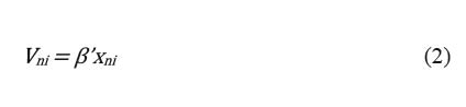
Vni depend on the attributes of the alternatives (xni) and on the fixed vector of coefficients (β’). The probability that the n-th farmer chooses the i-th alternative from choice set J is:
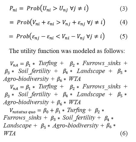
where variables have been described above (see Table 1).
As it concerns the stochastic part, we assumed an identically independently (IID) extreme value distribution. Consequently, equation (5) resulted in the choice probability of the Multinomial logit (MNL) model (McFadden, 1974):

Standard MNL implies homogeneity among individual preferences. As this assumption is strongly restrictive, particularly where heterogeneity has been already proven (Espinosa-Goded et al., 2010; Ruto and Garrod, 2009), we relaxed homogeneity assumption through the Mixed logit (MXL) (McFadden and Train, 2000; Train, 2003) in which the utility is modelled as follows:

where: β is the vector of mean attribute utility weights in the population; ηn is the vector of person n-specific deviations from the mean; ηn is a random parameter that accommodates the presence of unobservable preference heterogeneity in the sample (Hensher et al., 2015). The density of η is denoted as f (η|θ), where θ is the fixed parameter of the distribution. Given that the error term is assumed to be distributed as IID extreme value, for a given value of η, the conditional choice probability assumes a logit form:
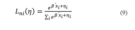
The term η is unknown. Consequently, it is possible to estimate the unconditional choice probability as the integral of (9) over all values of η, weighted by its density:
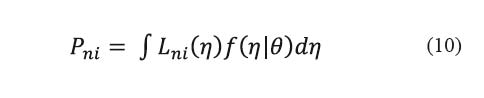
Since no simple closed-form solution exists for (10), calculations are accomplished by using numerical methods. This means that for any given value of θ, a value of η is drawn from f (η|θ) for R times, and the logit formula is calculated for R times as Lni(ηr), and finally averaged as demonstrated in the following equation:
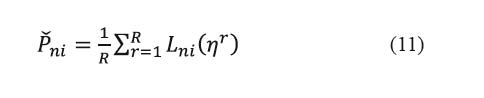
For random parameters, we assumed they are normally distributed; simulation was conducted through 1,000 random draws.
To verify if spatial variability in preferences for attributes were significant at local scale (Wilson and Hart, 2000; Birol et al., 2006; Campbell et al., 2009; Ruto and Garrod, 2009; Espinosa-Goded et al. 2010; Vergamini et al., 2013; Czajkowski et al., 2017), we used the Moran’s I test (Moran, 1950; Li et al., 2007; Yu et al., 2017). To further detect spatial autocorrelation, we also estimated non-spatial regression models, and tested for spatial dependence in the data set through Moran’s and Lagrange Multiplier robust tests on the residuals (Anselin, 2013; Yu et al., 2017). In these regression models, as dependent variable, we used MXL individual beta parameters with a significant random distribution; in the regressors, we included the farm’s cropped surface (in ha), the type of production process (conventional or organic), the familiarity with agro-environmental contracts, the educational level, the family size, the farming experience, and the land ownership.
For attributes presenting significant spatial correlation, we implemented a Spatial Autoregressive (SAR) model, which assumes that spatial dependencies exist directly among the levels of the dependent variable, and a Spatial Error (SEM) model, which assumes that spatial dependencies exist in the error term. These models were specified as follows:
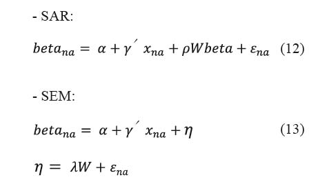
where betana is the parameter estimated through the MXL model for the n-th farmer respect the a-th attribute or level in case of dummy variables; α is an intercept term; γ is a vector of parameters for the observed explanatory variables xna to be estimated; W is a queen-based contiguity weight matrix; ρ is the spatial autoregressive coefficient, a scalar parameter that measures the magnitude of the spatial correlation in the spatial lag model; λ is a scalar parameter that measures the magnitude of the spatial correlation in the spatial error model; and εna is the idiosyncratic (normally distributed, homoscedastic, and uncorrelated) error term.
4. Results and discussion
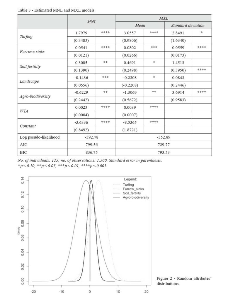
Table 3 reports estimates of MNL and MXL models. In the MNL model, all attributes were statistically significant, even though at different level of significance, and their signs were coherent with economic theory and expectations. Variables representing practices aimed at controlling the risk of soil erosion (Turfing and Furrows sinks) were highly significant (p < 0.001) and shown a positive sign. Turfing sloping surfaces is preferred to the realization of furrows-sinks because this practice assures a higher level of protection against water erosion. Coherently, in the hypothesis of furrows sinks, the realization of more closed sinks is preferred. The coefficient of Soil_fertility showed a lower significance level (p < 0.05) and was positive, meaning that the practice of grazing stubble and firebreaks was preferred to the creation of firebreaks and burying of crop residues, and that the creation of firebreaks and burying of crop residues was preferred to the burning of crop residues. The improvement in the degree of maintenance of the countryside features (Landscape) presented a higher level of significance (p < 0.01) and was negative due to the effort (which is also economic) that is not accompanied by additional revenues. The increase of the surface dedicated to crop local endangered varieties (Agro-biodiversity) negatively affected the farmer’s utility (p < 0.05) because it implies a lesser yield when compared with commercial crop varieties. The coefficient of WTA was highly significant (p < 0.001) and positive, meaning that the farmer’s utility increases with higher compensation. The constant term (β0), which represents the Alternative Specific Constant (ASC) for the status quo alternative, was negative and highly significant (p < 0.001). This result was coherent with that obtained by similar studies, confirming the farmers’ preference for the non-status quo alternative (Birol et al., 2006; Espinosa-Goded et al., 2010).
As it concerns MXL model, results confirmed our hypothesis of heterogeneous farmers’ preferences for agri-environmental practices. The better statistical performance was shown by the specification where attributes’ coefficients – except the coefficient of WTA – were randomly and normally distributed. The z value of standard deviation (Hensher et al., 2015; Mariel et al., 2013) rejected the hypothesis that the parameter for Landscape variable was randomly distributed. Figure 2 displays the distribution of the four random parameters having a standard deviation statistically significant.
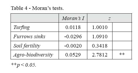
Table 4 reports estimates of Moran’s I tests on the MXL significant random parameters. Results indicated a significant and positive spatial autocorrelation only for the coefficient relative to Agro-biodiversity conservation, with a level of significance equal to 0.05.
Spatial diagnostic tests were reported in Table 5. Values of Moran’s I statistics on residuals confirmed previous results of Moran’s I test. The statistic shown a positive and statistically significant spatial correlation only for Agro-biodiversity (p < 0.10). Robust Lagrange Multiplier (LM) test statistics (spatial lag and spatial error) were both statistically significant for the same attribute, pointing out spatial autocorrelation in the dependent variable and in the error term. The level of significance of LM robust tests indicated a better statistical performance for the SAR model specification.
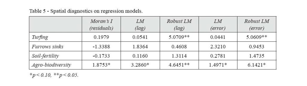
Table 6 reports estimates of full and restricted standard regression, and estimates of spatial regression models to analyse variability only for Agro-biodiversity conservation practices. In the estimation process, the beta value for this attribute was considered in absolute value. Restricted models were obtained adopting a stepwise backward-elimination approach (Harrell, 2015), which implies removing variables that are highly insignificant (p-value higher than 20%). Akaike info and Schwarz criterions assumed systematically lower values for restricted models, showing better statistical performances for these model specifications. Estimated signs shown a significant and negative relationship between the dependent variable and the practice of organic production process. This result is consistent with the economic features of organic enterprise and the low yield charactering the old varieties. The farmers’ experience influenced in a significant and positive way the crop of ancient local varieties. Preferences heterogeneity for biodiversity conservation did not depend on farmer’s age, educational level, ownership of land, familiarity with agri-environment schemes, and farmland size. These results contrast with those obtained in similar studies on the determinants of farmers’ preference heterogeneity for AES (Birol et al., 2006; 2009). However, these studies did not treat spatial patterns.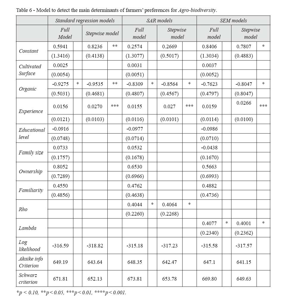
As it concerns spatial patterns, in the SAR model the coefficient ρ was statistically significant (p < 0.10). In the SEM model the coefficient λ was also statistically significant (p < 0.10). These results made inconclusive the choice between the SAR and the SEM model specifications.
5. Concluding remarks
Understanding in advance farmer’s preferences for environmental friendly practices is useful to design effective AES and promote sustainable agriculture in sensitive areas. In this study, we implemented a DCE exercise to generate information about farmers’ preferences among alternative AES designed to reduce soil risk of erosion, maintain soil fertility, enhance countryside landscape, and preserve agrobiodiversity in arable lands of Sicily.
We also investigated farmers’ preference heterogeneity and assessed the role played by the spatial correlation in the explanation of observed preference heterogeneity.
General findings indicated that farmers were aware on the rules of eco-conditionality locally in force, and positively welcomed the opportunity to exercise more restrictive eco-friendly agricultural practices. This availability, which is consistent with related literature, was statistically demonstrated by the sign assigned to the status quo alternative.
As it concerns the content of AES simulated in the experiments, we observed that farmers stated positive preference towards the maintenance of soil fertility and the control of the risk of soil erosion. In particular, turfing sloping surfaces was preferred to furrows-sinks. Among furrows sinks, farmers declared to prefer more closed sinks. In relation to practices aimed at protecting soil fertility, grazing stubble was considered the most appropriate respect to firebreaks, burying and burning crop residues. Practices to protect soil from water erosion and to maintain its fertility influenced positively the choice among alternative AES. Conversely, farmers perceived negatively the maintenance of countryside landscape elements, and the cultivation of old local varieties of grains. Dislike towards the crop of “ancient seeds” were correlated with organic farmers.
Estimates revealed also that farmers’ preferences were heterogeneous respect to the protection of soil from water erosion, the maintenance of soil organic matter, and the cultivation of local endangered varieties.
Spatial econometric analysis revealed that only preferences for agrobiodiversity conservation practices were positively auto-correlated among neighbors. The existence of a “neighbor effect” influencing farmers’ preferences for the cultivation of endangered varieties can be considered the main finding of the study. It suggests that in design AES, policy makers should account that famer’s preferences vary among practices but also among local contexts. Focus on local context might improve the acceptability of AES and achieve cost-effectiveness goals.
To conclude, we believe that policy makers could benefit from the empirical evidence provided by our study, especially in Mediterranean areas where the risk of desertification, and loss of agrobiodiversity is shifting to higher level as a consequence of climate change. AES remain the main tools to mitigate damages and promote sustainable agriculture. Our study reveal that AES currently in force do not fully capture the availability of farmers to increase their committment to protect land and environmental resources, and heterogeneity and local spatial pattern in preferences.
References
- Anselin L., 2013. Spatial econometrics: methods and models (Vol. 4), Springer Science & Business Media.
- Aslam U., Termansen M., Fleskens L., 2017. Investigating farmers’ preferences for alternative PES schemes for carbon sequestration in UK agroecosystems. Ecosystem Services, 27: 103-112.
- Bamière L., Havlík P., Jacquet F., Lherm M., Millet G., Bretagnolle V., 2011. Farming system modelling for agri-environmental policy design: the case of a spatially non-aggregated allocation of conservation measures. Ecological Economics, 70(5): 891-899.
- Bateman I., Carson R.T., Day B., Hanemann W.M., Hanley N., Hett T., Jones A., Loomes G., Mourato S., Ozdemiroglu E., Pearce D.W., Sugden R., Swanson J., 2002. Economic valuation with stated preferences techniques. a manual. Cheltenham, England: Edward Elgar Publishing.
- Beharry-Borg N., Scarpa R., 2010. Valuing quality changes in Caribbean coastal waters for heterogeneous beach visitors. Ecological Economics, 69(5): 1124-1139.
- Birol E., Smale M., Gyovai Á., 2006. Using a choice experiment to estimate farmers’ valuation of agrobiodiversity on Hungarian small farms. Environmental and Resource Economics, 34(4): 439-469.
- Birol E., Villalba E.R., Smale M., 2009. Farmer preferences for milpa diversity and genetically modified maize in Mexico: a latent class approach. Environment and Development Economics, 14(4): 521-540.
- Boncinelli F., Riccioli F., Casini L., 2017. Spatial structure of organic viticulture: evidence from Chianti (Italy). New Medit, 16(2): 55-63.
- Brady M., Irwin E., 2011. Accounting for spatial effects in economic models of land use: recent developments and challenges ahead. Environmental and Resource Economics, 48(3): 487-509.
- Broch S.W., Vedel S.E., 2012. Using choice experiments to investigate the policy relevance of heterogeneity in farmer agri-environmental contract preferences. Environmental and Resource Economics, 51(4): 561-581.
- Campbell D., Hutchinson G., Scarpa R., 2009. Using choice experiments to explore the spatial distribution of willingness to pay for rural landscape improvements. Environment and Planning A, 41(1): 97-111.
- Chaikaew P., Hodges A.W., Grunwald S., 2017. Estimating the value of ecosystem services in a mixed-use watershed: A choice experiment approach. Ecosystem Services, 23: 228-237.
- Christensen T., Pedersen A.B., Nielsen H.O., Mørkbak M.R., Hasler B., Denver S., 2011. Determinants of farmers’ willingness to participate in subsidy schemes for pesticide-free buffer zones-a choice experiment study. Ecological Economics 70(8): 1558-1564.
- Cooper J., Signorello G., 2008. Farmer premiums for the voluntary adoption of conservation plans. Journal of Environmental Planning and Management, 51(1): 1-14.
- Costedoat S., Koetse M., Corbera E., Ezzine-de-Blas D., 2016. Cash only? Unveiling preferences for a PES contract through a choice experiment in Chiapas, Mexico. Land Use Policy, 58: 302-317.
- Czajkowski M., Budziński W., Campbell D., Giergiczny M., Hanley N., 2017. Spatial heterogeneity of willingness to pay for forest management. Environmental and Resource Economics, 68(3): 705-727.
- Defrancesco E., Gatto P., Runge F., Trestini S., 2008. Factors affecting farmers’ participation in agri-environmental measures: a northern Italian perspective. Journal of agricultural economics, 59(1): 114-131.
- Drechsler M., Wätzold F., Johst K., Bergmann H., Settele J., 2007. A model-based approach for designing cost-effective compensation payments for conservation of endangered species in real landscapes. Biological conservation, 140(1-2): 174-186.
- Dupraz P., Vermersch D., De Frahan B.H, Delvaux L., 2003. The environmental supply of farm households: a flexible willingness to accept mode. Environmental and Resource Economics, 25: 171-189.
- El Amami H., Fouzai A., Jamel N.A.S.R., Bachta M.S., 2013. Impact économique de la protection des sols à l’amont des bassins sur l’agriculture irriguée à l’aval: Analyse par l’approche Target MOTAD. New Medit, 12(2): 57-65.
- Espinosa-Goded M., Barreiro-Hurlé J., Ruto E., 2010. What do farmers want from agri-environmental scheme design? a choice experiment approach. Journal of Agricultural Economics 61(2): 259-273.
- Felardo J., Berrens R., 2018. Heterogeneous attitudes towards a payment for ecosystem services program. International Journal of Ecological Economics and Statistics, 39(1): 112-131.
- Galdeano-Gomez E., Zepeda-Zepeda J.A., Piedra-Munoz L., Vega-Lopez L.L., 2017. Family farm’s features influencing socio-economic sustainability: An analysis of the agri-food sector in southeast Spain. New Medit, 16(1): 50-62.
- Greiner R., Bliemer M., Ballweg J., 2014. Design considerations of a choice experiment to estimate likely participation by north Australian pastoralists in contractual biodiversity conservation. Journal of choice modelling, 10: 34-45.
- Harrell F.E., 2015. Multivariable modeling strategies, In: Regression modeling strategies. Cham: Springer.
- Hensher D.A., Rose J.M., Greene W.H., 2015. Applied choice analysis. A Primer, second edition. Cambridge: Cambridge University Press.
- Hynes S., Garvey E., 2009. Modelling farmers’ participation in an agri-environmental scheme using panel data: an application to the rural environment protection scheme in Ireland. Journal of Agricultural Economics, 60(3): 546-562.
- Jaeck M., Lifran R., 2009. Preferences, norms and constraints in farmers’ agro-ecological choices. case study using a choice experiments survey in the Rhone River Delta, France, paper presented at the 53rd Australian Agricultural and Resource Economics Society (AARES), Cairns (Australia), February 11-13.
- Li H., Calder C.A., Cressie N., 2007. Beyond Moran’s I: testing for spatial dependence based on the spatial autoregressive model. Geographical Analysis, 39(4): 357-375.
- Lienhoop N., Brouwer R., 2015. Agri-environmental policy valuation: farmers’ contract design preferences for afforestation schemes. Land-Use Policy, 42: 568-577.
- Louviere J.J, Henser D.A, Swait J.D., 2000. Stated Choice Method: Analysis and Application. Cambridge: Cambridge University Press.
- Mariel P., De Ayala A., Hoyos D., Abdullah S., 2013. Selecting random parameters in discrete choice experiment for environmental valuation: a simulation experiment. Journal of choice modelling, 7: 44-57.
- Matta J.R., Alavalapati J.R., Mercer D.E., 2009. Incentives for biodiversity conservation beyond the best management practices: are forestland owners interested? Land Economics, 85(1): 132-143.
- McFadden D., 1974. The measurement of urban travel demand. Journal of public economics, 3(4): 303-328.
- McFadden D., 2001. Economic choices. The American Economic Review, 91(3): 351-378.
- McFadden D., Train K., 2000. Mixed MNL models for discrete response. Journal of applied Econometrics, 447-470.
- McWilliam W., Fukuda Y., Moller H., Smith D., 2017. Evaluation of a dairy agri-environmental programme for restoring woody green infrastructure. International Journal of Agricultural Sustainability, 1-15.
- Moran P.A.P., 1950. Notes on continuous stochastic phenomena. Biometrika, 37(1): 17-23.
- Mulatu D.W., van der Veen A., van Oel P.R., 2014. Farm households’ preferences for collective and individual actions to improve water-related ecosystem services: The Lake Naivasha basin, Kenya. Ecosystem services, 7: 22-33.
- Mullan K., Kontoleon A., 2012. Participation in payments for ecosystem services programmes: Accounting for participant heterogeneity. Journal of Environmental Economics and Policy, 1(3): 235-254.
- Muradian R., Corbera E., Pascual U., Kosoy N., May P.H., 2010. Reconciling theory and practice: An alternative conceptual framework for understanding payments for environmental services. Ecological economics, 69(6): 1202-1208.
- Nyongesa J.M., Bett H.K., Lagat J.K., Ayuya O.I., 2016. Estimating farmers’ stated willingness to accept pay for ecosystem services: case of Lake Naivasha watershed payment for ecosystem services scheme-Kenya. Ecological Processes, 5(1): 15.
- Raes L., Speelman S., Aguirre N., 2017. Farmers’ preferences for PES contracts to adopt silvopastoral systems in southern Ecuador, revealed through a choice experiment. Environmental management, 60(2): 200-215.
- Randrianarison H., Ramiaramanana J., Wätzold F., 2017. When to pay? adjusting the timing of payments in PES design to the needs of poor land-users. Ecological Economics, 138: 168-177.
- Rocchi L., Paolotti L., Fagioli F.F., 2017. Defining agri-environmental schemes in the buffer areas of a natural regional park: An application of choice experiment using the latent class approach. Land Use Policy, 66: 141-150.
- Ruto E., Garrod G., 2009. Investigating farmers’ preferences for the design of agri-environment schemes: a choice experiment approach. Journal of Environmental Planning and Management, 52(5): 631-647.
- Santos R., Clemente P., Brouwer R., Antunes P., Pinto R., 2015. Landowner preferences for agri-environmental agreements to conserve the montado ecosystem in Portugal. Ecological Economics, 118: 159-167.
- Schulz N., Breustedt G., Latacz-Lohmann U., 2014. Assessing farmers’ willingness to accept “greening”: Insights from a discrete choice experiment in Germany. Journal of agricultural economics, 65(1): 26-48.
- Tesfaye A., Negatu W., Brouwer R., Zaag P., 2014. Understanding soil conservation decision of farmers in the Gedeb watershed, Ethiopia. Land Degradation & Development, 25(1): 71-79.
- Train K., 2003. Discrete choice methods with simulation. Cambridge: Cambridge University Press.
- Vaissière A.C., Tardieu L., Quétier F., Roussel S., 2017. Preferences for biodiversity offset contracts on arable land: a choice experiment study with farmers, paper presented at the 23rd EAERE Annual Conference, Athens (Greece), 28 June – 01 July, 2017.
- Vanslembrouck I., Huylenbroeck G., Verbeke W., 2002. Determinants of the willingness of Belgian farmers to participate in agri-environmental measures. Journal of agricultural economics, 53(3): 489-511.
- Vedel S.E., Jacobsen J.B., Thorsen B.J., 2010. Contracts for environmental goods and the role of monitoring for landowners’ willingness to accept. In: World conference of environmental and resource economics, Montreal, Canada.
- Vergamini D., Raggi, M., Viaggi, D., 2013. Optimal targeting and payment design for Agri-Environmental Measures: A resource allocation model for Emilia Romagna (Italy), paper presented at the 54th Annual Scientific Meeting of the Italian Society of Economists (SIE), Bologna, 24-26 October, 2013.
- Villanueva A.J., Rodríguez-Entrena M., Arriaza M., Gómez-Limón J.A., 2017. Heterogeneity of farmers’ preferences towards agri-environmental schemes across different agricultural subsystems. Journal of environmental planning and management, 60(4): 684-707.
- Vorlaufer T., Falk T., Dufhues T., Kirk M., 2017. Payments for ecosystem services and agricultural intensification: Evidence from a choice experiment on deforestation in Zambia. Ecological Economics, 141: 95-105.
- Wätzold F., Drechsler M., 2005. Spatially uniform versus spatially heterogeneous compensation payments for biodiversity-enhancing land-use measures. Environmental and Resource Economics, 31(1): 73-93.
- Whittington D., Pagiola S., 2012. Using contingent valuation in the design of payments for environmental services mechanisms: a review and assessment. The World Bank Research Observer, lks004.
- Wuepper D., Heissenhuber A., Sauer J., 2017. Investigating rice farmers’ preferences for an agri-environmental scheme: Is an eco-label a substitute for payments? Land Use Policy, 64: 374-382.
- Yu T.E., Lambert D.M., Cho S.H., Koc A.A., Boluk G., Kim S.G., 2017. A spatial analysis of the relationship between agricultural output and input factors in Turkey. New Medit, 16(1): 11-17.
- Zandersen M., Oddershede J., Pedersen A.B., Nielsen H.Ø., Termansen M., 2016. Payment for ecosystem services-paying farmers for using farmland for flood control. In: Adaptation Futures.