The use of crowdsourced geographic information for spatial evaluation of cultural ecosystem services in the agricultural landscape: the case of Chianti Classico (Italy)

Abstract

The use of geo-tagged photographs seems to be a promising alternative to assess Cultural Ecosystem Services CESs in respect to the traditional investigation when focusing on the study of the aesthetic appreciation of a protected area or natural landscape. The aim of this study is integrating the cumulative viewshed calculated from geotagged photo metadata publicly shared on Flickr with raster data on infrastructure, historical sites, and the natural environment, using landscape ecology metrics and RandomForest modelling. Crowdsourced data provided empirical assessments of the covariates associated with visitor distribution, highlighting how changes in infrastructure, crops and environmental factors can affect visitor’s use. These data can help researchers, managers, and public planners to develop projects, and guidelines in the rural landscape for incresing the supply for CESs.

DOI: 10.30682/nm1902g

Veronica Alampi Sottini*, Elena Barbierato*, Iacopo Bernetti*, Irene Capecchi*, Sara Fabbrizzi*, Silvio Menghini*

* University of Florence, Department of Agricultural, Food and Forestry Systems (GESAAF), Firenze (Italy).

Corresponding author: iacopo.bernetti@unifi.it

Download PDF

Cite this Item: Alampi Sottini V., Barbierato E., Bernetti I., Capecchi I., Fabbrizzi S., Menghini S., 2019. The use of crowdsourced geographic information for spatial evaluation of cultural ecosystem services in the agricultural landscape: the case of Chianti Classico (Italy), New Medit, 18 (2): pp. 105-118, http://dx.doi.org/10.30682/nm1902g

1. Introduction

The importance of Cultural Ecosystem Services (CESs) to human well-being is widely recognised. However, quantifying these intangible benefits is difficult and thus it is often not assessed. Mapping approaches are increasingly used to understand the spatial distribution of different CESs, as well as to analyse how they are related to landscape characteristics and rural activities. CESs represent the intangible benefits that people receive from ecosystems through cultural heritage, spiritual enrichment, recreation and tourism, and aesthetic experiences. They are considered fundamental to well-being and are often at the heart of discussions on the protection of ecosystems (Bullock et al., 2018). CESs represent a framework that contribute to integrate the different types of ecosystem services delivery and biodiversity conservation of the agroecosystems into synergistic strategies (Mace et al., 2012; Assandri et al., 2018); however, CESs very often fall victims to policy makers’ preferences for economic, social or ecological values, as they are not included in economic evaluation and landscape planning., (Mileu et al., 2013; Winkler and Nicholas, 2016). Based on the existing features and traditions, promotion of tourism and recreation is a preferred rural development option (Van Berkel and Verburg, 2014) creating opportunities to convert a part of the externalities produced in agriculture in productive resources for the sector and, consequently, inducing strong synergies between the economic and the socio-environmental objectives. In particular, vineyard landscape provides several Cultural Ecosystem services, such as cultural heritage values, aesthetic values and recreational opportunities (Winkler et al., 2017). The mapping of the preferred locations in the landscape allows for statistical and spatial analysis to be conducted to determine the relative importance of different factors for the delivery of CESs, considering the fundamental role of agriculture. Most studies evaluating ecosystem services have been limited to quantifying recreation and tourism, leaving out the intrinsic qualities that are interrelated with tourism in the cultural service category.

Some advances have been recently provided by Big Data and, specifically, by social media analysis. The use of geo-tagged photographs seems to be a promising alternative to assess CES in respect to the traditional investigation when focusing on the study of the aesthetic appreciation of a protected area or natural landscape (Tenerelli et al., 2016; Schirpke et al., 2017; Levin et al. 2017; Yoshimura and Hiura 2017; Walden-Schreiner et al. 2018).

The aim of this study is integrating the cumulative viewshed calculated from geotagged photo metadata publicly shared on Flickr with raster data on infrastructure, historical sites, and the natural environment, using landscape ecology metrics and RandomForest modelling. Crowdsourced data provided empirical assessments of the covariates associated with visitor distribution, highlighting how changes in infrastructure, crops and environmental factors can affect visitor’s use. These data can help researchers, managers, and public planners to develop projects, standards, and guidelines in the rural landscape, underlying how the evolution of the agricultural activities, and their land use, can influence their public contribution to the CESs. The results of the research of Torquati, Giacché and Venazi (2015) «indicate that in some contexts the preservation of the landscape can become an interesting marketing vehicle, enabling wine growers who produce quality wines to increase their income. This result demonstrates that landscape preservation can be a driving force for improvements in farm management and farm income, much more effective than the establishment of protected landscapes, and it confirms the importance of traditional landscapes as a driver of rural development».

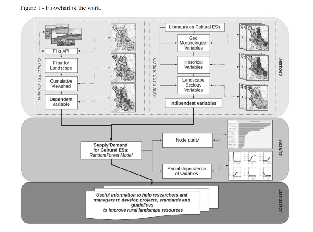
Figure 1 shows the graphical abstract of the paper. The first phase of the work involved the development of two geodatabases. The first database is related to the demand for ecosystem services through the calculation of cumulative viewshed from the points from which the photos of agricultural landscapes shared on Flickr were taken. The second geodatabase relates to the ecological and historical landscape variables that make up the territorial offer of ecosystem services. Supply and demand were spatially modelled to assess the importance of different variables using a Random Forest model. By implementing the methods of the partially dependent areas and the thematic contribution areas it was possible to obtain very precise indications on the policies for the conservation and enhancement of the cultural ESs of the Chianti area.

2. Study area

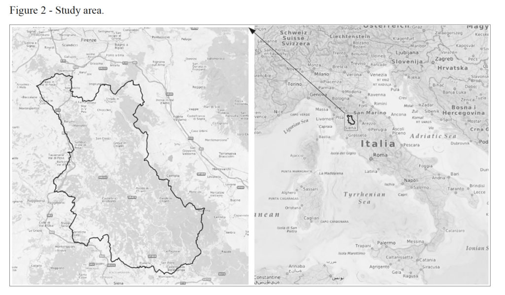
The territory of the appellation of the Chianti Classico (Figure 2) extends for 71,800 hectares located between the provinces of Siena and Florence. The characteristics of the climate, the soil and the different altitudes make the Chianti area a region suited to produce quality wines. The characteristic element of the Chianti agricultural landscape are the rows of vines that alternate with the olive groves. With over 7,200 hectares of vineyards registered in the D.O.C.G. register, Chianti Classico is one of the most important appellations in Italy. The enhancement of the territory and landscape of Chianti has its origins since the sixteenth century when, with the conversion of the Florentine Lordship into the Grand Duchy of Tuscany, banking and commercial activities went into crisis and many investments were directed to strengthening the primary production. Some forms of production still present today originated from that period (Marone and Menghini, 1991).

Torquati, Giacché and Venanzi (2015, p. 122) have defined Chianti as a «Traditional Cultural Vineyard Landscape (TCVL) because the viticulture sector is the one most integrated with the kind of tourism that is interested in quality food products associated with a specific place of origin, and also the sector that, more than others, has responded to market changes by increasing the appeal of their products».

Vineyards are one of the most powerful territorial markers as they act as carriers of rural identity. The typical landscape of Chianti reflects itself in the highly specialized wine production. Even the most inexperienced observer can easily recognize the link between the landscape and the typical product of the area. These two specific characteristics allow us to go beyond the concept of TCVL towards a viticultural landscape, underlining the relations between the final product (the wine) and the territory, thus bringing the well-known opportunities for commercial differentiation that in the sector are defined in the concept of terroir and in specific production areas with an appellation of origin.

3. Methods

3.1. Demand for CESs

According to the scientific literature, demand for CESs can be estimated from the territorial density of the shooting points of the photos published on Flickr. Photo sharing sites, such as Flickr, allow users to cloud storage the photos and to view the geotagged and map-based photo locations. Studies also indicate that Flickr data can be spatially accurate and timely. Many studies showed that the number of uploaded photos was positively correlated with other methods of monitoring visitors and that it could be used to provide information on the movements, itinerary and distribution of the visitors.

Using an algorithm based on Flickr’s Application Programming Interface, the coordinates of the shooting points of shared photos from 2005 to 2017 were downloaded. The photos containing the tags “wine”, “vineyard”, “Chianti”, and related words, were filtered. Then, specific filters were applied to avoid distortions due to photos being repeated several times in a single location by a single photographer. The records were downloaded and analysed in R and converted into shapefiles for geospatial analysis using QGIS.

When analysed in combination with spatial data, the spatial patterns of photo density can reveal the preference for different landscape attributes (Van Zanten et al., 2016) or the consequences of land-use change (Sonter et al., 2016). From the point of view of statistical modelling, the most used approach is the Maximum Entropy model (Braunisch et al., 2011; Westcott and Andrew, 2015; Coppes and Braunisch, 2013; Richards and Friess, 2015; Yoshimura and Hiura, 2017; Walden-Schreiner et al., 2018). Recently Tenerelli, Püffel and Luque (2017) used the cluster analysis to integrate visual characters of the landscape and visiting users’ preferences and Van Berkel et al. (2018) developed a model where the response variable is assumed to follow a negative binomial (NB) distribution.

These studies allowed us to take advantage of social media for analysing landscape preferences. However, the different approaches still show some limitations as for the setting up of a decision support system, of projects and plans for the preservation and for the development of cultural ecosystem services of the rural landscape. The approaches based on the probabilistic models (MaxEnt and NB distribution) relate the probability of having a preference on a landscape (that leads to a photo shared on Flickr) with the territorial characteristics that occur in a single pixel or in its close spatial proximity. The photographic recovery, on the other hand, is influenced by the entire surrounding landscape (Van Berkel et al., 2018). In this regard, the calculation of the viewshed is a potentially useful geographic instrument able to capture the perception of the landscape. A viewshed is the 360° area that is visible from a discrete location (Vukomanovic et al., 2018). It includes all the surrounding points within the line-of-sight of an assumed viewer’s location and excludes points that are obstructed by the terrain or by other features. Viewshed research has been instrumental to the understanding of the scenic values associated with residential development (Vukomanovic and Orr, 2014) and to the relationship between aesthetic values and landscape patterns (Schirpke et al., 2016). However, the difficulty in identifying the subject of appreciation within the viewshed has unfortunately led many studies to resort to the best guess regarding the precise location of the appreciated areas (Schirpke et al., 2016; Yoshimura and Hiura, 2017). Combining georeferenced photos provided voluntarily by social media users with viewshed analysis represents a unique opportunity to evaluate the landscape qualities and visible attributes associated with highly valued areas.

In our work, as a proxy for the demand for CESs, an index using cumulative viewsheds calculated from photographing positions was developed. Visibility analysis is increasingly implemented by landscape planners in effective decision support systems for the best possible spatial arrangement of land uses and for assessing the visual impact of certain features on the landscape (Palmer and Hoffman, 2001; Bell, 2001; Bryan, 2003; Hernández et al., 2004). Perhaps the most popular concept used to explore visual space in a landscape has been the cumulative viewshed (Wheatley, 1995; Martín Ramos and Otero Pastor, 2012), sometimes called total viewshed or intrinsic viewshed (Franch-Pardo et al., 2017). In general, cumulative viewsheds are created by repeatedly calculating the viewshed from various viewpoint locations, and then adding them together one at a time using the map algebra to produce a single image. We defined and calculated each viewshed using a 10 m digital DTM from a height of 165 cm and within a maximum radius of 5 km (Willemen et al., 2008; Chesnokova, Nowak and Purves, 2017; Bradbury et al., 2018). To obtain a cumulative viewshed, the single viewsheds were added together. The result was transferred into a hexagonal grid theme with a cell size of 1 km (Willemen et al., 2008; Chesnokova, Nowak and Purves, 2017; Bradbury et al., 2018) with visibility attributes assigned to each cell.

3.2.The potential supply of CESs

We define potential supply as the set of intrinsic territorial characteristics that contribute to determining the offer of cultural ecosystem services. Potential supply differs from the real one as it includes locations with intrinsic characteristics that can potentially satisfy demand, but at the same time it has limitations that do not allow the matching between supply and demand. The aim of the potential supply model is to identify these locations that represent the most interesting places for the development of targeted territorial policies.

It is possible to map the potential supply of CESs by analysing the relationship between the demand area and its environmental factors as the demand map represents the visitors’ aesthetic preferences.

Analysing the explanatory variables used in the different studies it is possible to highlight that:

- the model of Richards and Friess (2015) adopted four environmental factors: (1) the distance from the nearest footpath (including the boardwalk), (2) the distance from focal points (rest shelters and a viewing tower), (3) the distance from the site entrance, and (4) the dominant habitat type within the neighbouring 30 m;

- the model of Yoshimura, and Hiura (2017) used vegetation type, distances from rivers, lakes, or coastline as explanatory variables and 10 classes of topography features;

- Richards and Tunçer (2017) used four explanatory variables: (1) the distance from the nearest major out-door attraction, (2) the presence of parks, including nature reserves, (3) the proportional coverage of forest within 50 m, and (4) the proportional coverage of managed vegetation within 0.01 km, 2 grid squares;

- In the MaxEnt model used by Walden-Schreiner et al. (2018) visitor infrastructure (i.e., distance to buildings, parking, roads, trails, and campsites) and environmental characteristics (i.e., vegetation type, elevation, slope, and distance to water) served as independent variables.

Our approach for assessing CESs provided by viticultural landscapes is based on spatially explicit quantitative indicators mainly represented by landscape ecology metrics. The analysis of the relationships between the visual quality of the landscape and its structural properties is an active area of research in the field of environmental perception. For the assessment of landscape quality, reference was made to the exhaustive classification of indicators proposed by Ode, Tveit and Fry, 2008. The conceptual framework developed by these authors allows to link each indicator to concepts described by different aesthetic theories of landscape: (a) the concept of complexity can be explained by several theories that include the Biophilia evolutionary theory (Ulrich, Kellert and Wilson, 1993); (b) naturalness is related to the degree of naturality (or naturalness) of the environment observed and it is explained by the restorative and therapeutic role of nature (Kaplan, 1995); (c) historicity is linked to the presence of historical and temporal elements in the landscape and to man’s ability to recognize his identity in the landscape according to the theory of Genius Loci (Norberg-Schulz, 1980); (d) the concept of coherence is explained by the legibility aspects of the theories of Information Processing (Kaplan and Kaplan, 1989); (e) the concept of visual scale derives from the Evolutionary theory developed by Appleton (1996) that link preferences to the opportunity of prospect (ability to see) and refuge (not being seen).

According to the above, the following visual quality indicators were selected and were divided into five conceptual categories:

Complexity indicators:

number of different land cover per view;

Shannon index.

Naturalness indicators:

percentage area, edge density, and number of patches of natural and semi-natural vegetation;

percentage area, edge density, and number of patches of water bodies.

Historicity indicators:

distance from historic villages;

distance from historic roads.

Coherence indicators:

percentage area, edge density, and number of patches of vineyards;

percentage area, edge density, and number of patches of olive groves;

percentage area, edge density, and number of patches of arable land.

Visual scale indicators:

elevation, standard deviation of elevation, range of elevation.

According to the classification proposed by Ode et al., 2009, indicators related to the category of visual disturbance, also called indicators of lack of consistency (Kaplan and Kaplan, 1989), should also be considered. This category includes, for example, the density of modern buildings and infrastructures with a high visual impact. However, in the area under consideration these elements are absent or scarcely significant and are therefore not relevant for the definition of the potential supply.

The indicators were calculated at landscape level using the Frastag software. The maps of the indicators, such as the cumulative viewshed, were also sampled using a hexagonal grid. The hexagonal grid is recommended by the authors of the FRAGSTATS Patch Analyst implementation (McGarigal and Marks, 1995) as the form of stacking that, being closer to a circle, minimizes angular effects.

A non-parametric multivariate approach was used to determine the most important landscape variable to be associated with the cumulative viewshed variable. Non-parametric approaches do not assume normality in the distributions of the variables and, consequently, complex data are better analysed in this way. Since many metrics were evaluated, an ensemble decision tree approach was selected to regress biodiversity variables many times against all possible metrics using random forest regression (Breiman, 2001).

To estimate the spatial distribution of the potential supply of Cultural SEs, a RandomForest (RF) model was used with cumulative viewshed as the dependent variable and potential offer indicators as independent variables. RF is a popular and useful tool for non-linear multi-variate classification and regression, which produces a good trade-off between robustness (low variance) and adaptiveness (low bias). Direct interpretation of a RF model is difficult, as the explicit ensemble model of hundreds of deep trees is complex. In the case of linear regression, we can gain a remarkable understanding of the structure and interpretation of the model by examining its coefficients. For more complex models, such as random forests, a relatively simple parametric description is not available, which makes them more difficult to interpret. To overcome this difficulty Friedman (2001) proposed the use of partial dependence plots that allow visualizing a suitable RF model through its mapping from feature space to prediction space. Welling et al. (2016) propose a new methodology, forest floor, to first use feature contributions (FC), a method to decompose trees by splitting features and then performing projections. The advantages of forest floor over partial dependence plots is that interactions are not masked as averaging. As a result, interactions that are not visualized in a given projection can be located. Forest floor was implemented in the foresFloor library for the statistical programming language R.

4. Results

The raw database contained about 28,815 photo localizations taken in the period 2005-2017. Only photos taken in the rural landscape were selected for analysis. Subsequently, the pictures that contained the tags “wine”, “vineyard”, “Chianti” and related words, were filtered. Finally, specific filters were applied to avoid distortions due to photos repeated many times in a single location by a single photographer. The final dataset contained 9,304 photographic points.

Figure 3 shows a demand map based on the cumulative viewshed index. This map provides an overview and a detailed distribution of the aesthetic demand.

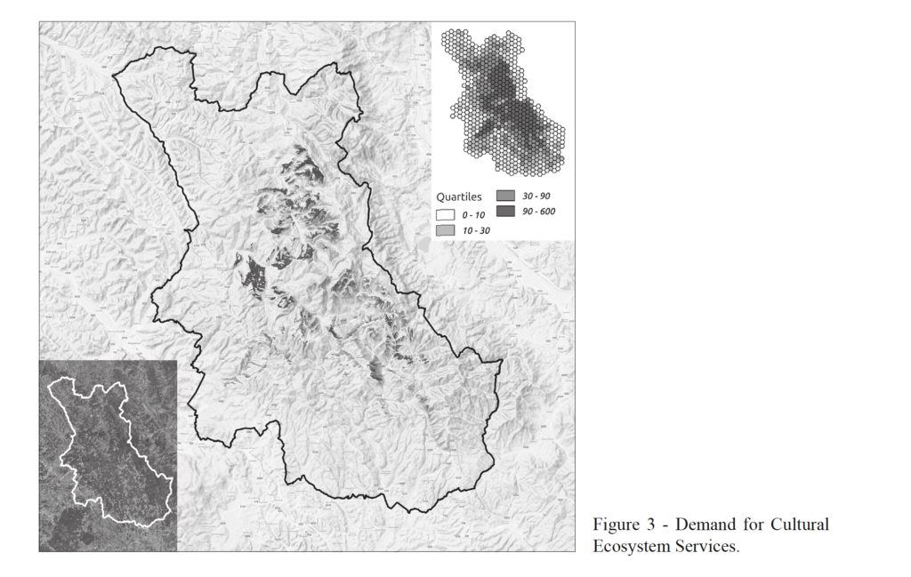
The cumulative viewshed index recorded a maximum value of 600 with an average value of 60 and a median value of 20, thus with a frequency distribution that is very asymmetrical. The areas with the highest demand for CES are in the cultivated hill characterized by a complex mosaic of vineyards, fields and wooded areas. Figure 4 shows the observed, predicted and relative error percentage values of the demand estimation model for Cultural ES. The figure shows that the most significant percentage errors are localized in areas with low demand (mainly at the edge of the map due to the weak effect of variables localized just outside the boundary of the area), confirming the reliability of the model in identifying the relevant environmental factors in the locations with the highest value.

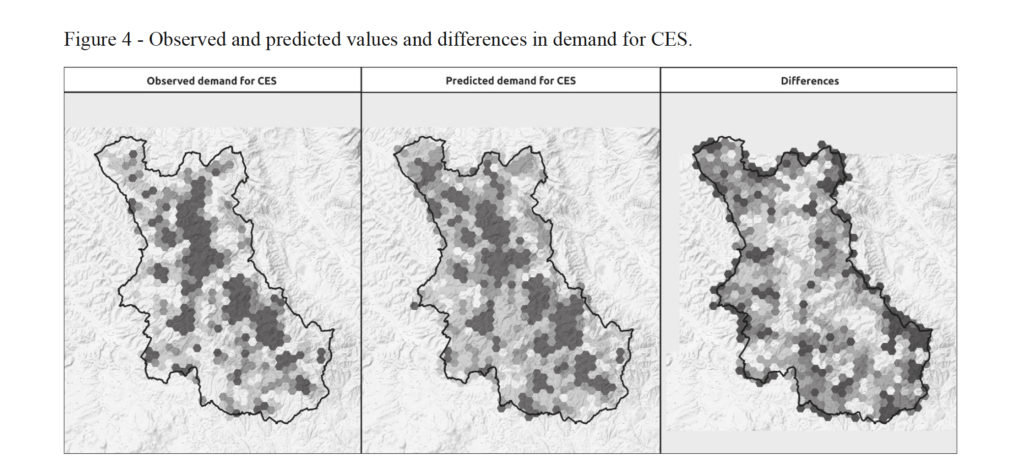
The pseudo R² of the Random Forest model was 0.89 so the predictive accuracy is considered high. Table 1 shows the environmental factors that contributed most to the model. In order, they were: distance from historic villages, percentage of forest, vineyard edge density, distance from historical path, percentage of heterogeneous agricultural areas and percentage of vineyards.

To understand the effect of the environmental characteristics on the demand for CESs the partial contribution graph of the characteristics is used. Figure 5 shows the FC plots of the 9 variables with the highest importance in the model.

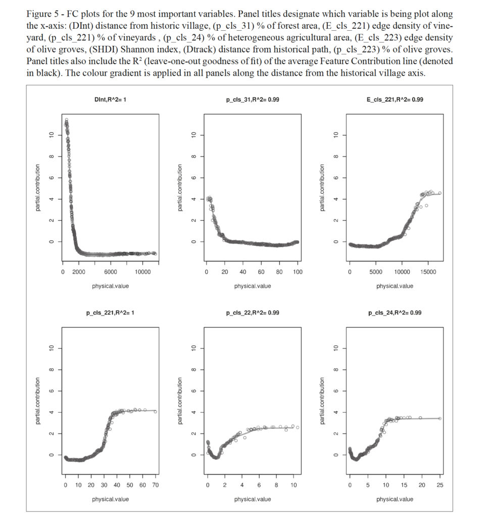
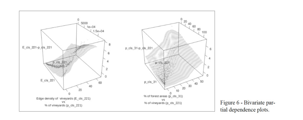
FC plots are very useful for understanding the effect of environmental characteristics on the demand for CESs. The analysis of the FC plot of the distance from historical villages allows assessing that the variable’s contribution to the demand for CES decreases as the distance increases and becomes irrelevant beyond 1,000 meters. The percentage of forest is inversely proportional to the demand for CESs too, as well as to the distance from the historical paths. On the other hand, the margin density of the vineyards is positively correlated with the demand for CES with optimal values between 10,000 and 15,000 meters of margin per hectare. The percentage of vineyard also makes a positive contribution up to a maximum limit of 40% of the total area. The FC graphs allow evaluating the interaction between two environmental variables. Figure 6 shows examples of bivariate FC charts: it can be noted that the cross combinations that most contribute to the demand for ESCs, are related to landscapes with up to 20% of forests and up to 50-60% of vineyards with a density of margins of 15,000 meters per hectare.

5. Discussion

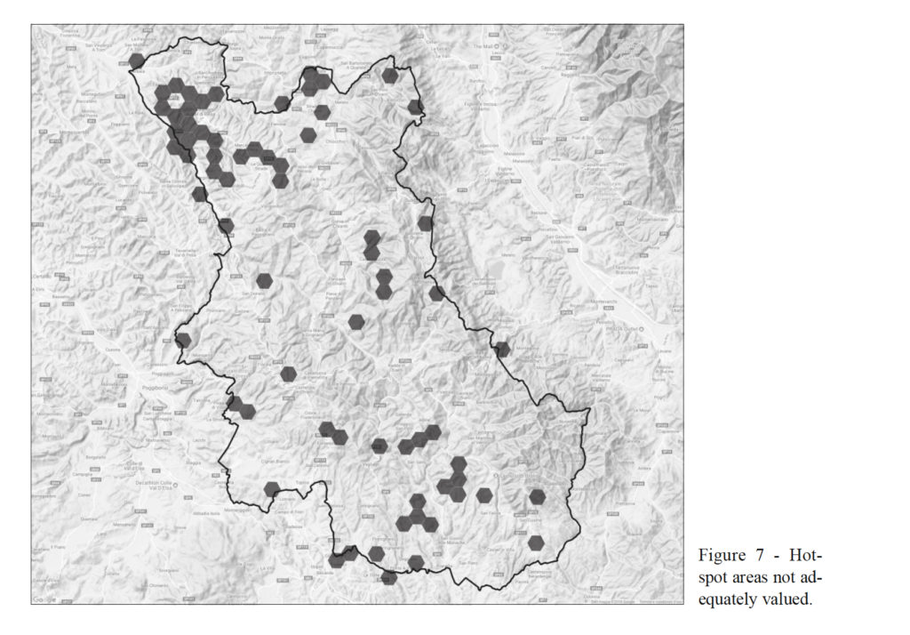
The results of the models highlight that vineyards and arable land separated by hedges and vegetation strips contribute to a higher value of CESs. The results indicate that approximately half of the variation in scenic perceptions can be explained by spatial landscape metrics. These results give landscape planners and designers some insight into the preferred composition and configuration of human landscapes. They provide additional support for the contribution of natural-appearing landscapes with a complex pattern of edges to the landscape quality of a community. The use of partial-dependent graphs also provides useful indications for rural policy interventions that maintain and/or increase the supply of ESCs, avoiding excessive specialization in land regulations, which are more difficult to manage. This aspect also involves the hydraulic arrangements of the slopes, on which practically the entire cultivation of vines develops in the area under examination. In addition, areas with a positive difference between the expected and observed values in the Randomforest model represent areas with a good probability of having a high potential CESs value. Figure 7 shows localizations with both high values (beyond the third quartile) in the observed demand for CESs and high percentage difference (above the third quartile) between observed and predicted demand. These localizations are hotspot areas not adequately exploited either because the tourist flows are external to them or because of the presence of visual detractors that could be removed through landscape restoration projects. On the other hand, for the locations shown in Figure 7, it is necessary to consider actions to increase the attractiveness of places, removing the limiting causes. For locations with both high values in the observed demand and minimal deviations between expected and observed values, safeguard and/or consolidation measures of an already satisfactory situation should be implemented. Lastly, localizations with a high value of the observed demand and a low value of the predicted demand represent places where there are landscape characteristics not considered by the present model, but which have a significant local importance. These characteristics must be identified singularly and safeguarded.

The models applied confirmed the importance of agricultural cultivations for the value of the landscape and allowed to obtain a spatial assessment of the consistency of the externalities produced by agriculture, providing clear benefits for the choices of territorial government and rural development. The analysis showed that the correlation between cumulative viewshed and the indicators of landscape ecology gives useful information for the definition of rural policies for the enhancement of rural landscape in Mediterranean region. The FC plot analysis allowed identifying the territorial relationship among historical buildings, roads and rural landscape elements, thus defining the localizations to be preserved and enhanced through events. The FC curves allowed the definition of specific agricultural land planning interventions. As an example, Figure 5 shows the FC curves for the following variables: percentage of vineyards, percentage of olive groves, edge density of olive groves, and edge density of vineyards; these curves allowed the outlining of a model of identity landscape consisting of a mosaic made with up to 20% of forests, up to 30-40% of olive grows and up to 30-40% of vineyards with a density of margins such as to lead to a Shannon Index of approximately 3.

6. Conclusion

The results of the work show that a reliable estimate of the demand for Cultural ESs can be assessed by calculating the cumulative viewshed from the shooting points of the photos shared on Flickr social media. This method is easily transferable to other territories with limited re-pricing costs. The relationship between the demand for Cultural ESs and the historical and environmental characteristics of the landscape can be effectively estimated through a Random Forest regression model. Moreover, the analysis of the results of the model implementing the Feature Contribution plots method allows having important and very detailed quantitative information for the implementation of rural policies to enhance the rural territory. As highlighted in the results, the model provides a useful analysis to distinguish those areas that already fully express their attractiveness from those that have a good potential but is still unexpressed.

Thanks to the spatialization of the results, the suggested model offers the planner the possibility of identifying the areas in which to intervene with priority implementing safeguard projects, starting from the containment of the anthropic pressure. At the same time, the model detects those areas in which it is necessary to stimulate a certain attractiveness, both in favour of primary production activities – which help to generate and maintain some essential landscape components – and in favour of external visitors. This study can stimulate further research aimed at detecting the perception of individuals on the ecosystem services that a landscape can provide, helping planners and policy makers to optimise choices for the effective management of the agricultural landscape (Sanchez-Zamora et al., 2014). In recent years, an increasing share of budgetary resources has been used for measures aimed at protecting the visual quality of agricultural landscapes (Howley et al., 2012). Thus, understanding of the perceptions of individuals on landscapes becomes an essential cognitive element for the effective planning of rural development policies, in line with the promotion of bottom-up approaches of territorial governance (De Vreese et al., 2016).

Lastly, the 2014-2020 CAP presented policies focused on the efficient provision of ecosystem services from agricultural land. The capacity of agroforestry practices to improve the provision of cultural ecosystem services can be encouraged through public policies such as the EU biodiversity strategy to 2020, but the separation between agriculture and forestry in the current EU perspective is a limit to a support framework for agroforestation. Therefore, the results of the present study can provide information for designing a new CAP with combined rural and forest planning measures.

References

Appleton J., 1996. The experience of landscape. Chichester: Wiley, pp. 66-67.
Assandri G., Bogliani G., Pedrini P. and Brambilla M., 2018. Beautiful agricultural landscapes promote cultural ecosystem services and biodiversity conservation. Agriculture, Ecosystems and Environment, 256: 200-210.
Bell S., 2001. Landscape pattern, perception and visualisation in the visual management of forests. Landscape and Urban planning, 54(1-4): 201-211.
Bradbury R., Ridding L.E., Redhead J.W., Oliver T.H., Schmucki R., McGinlay J., Graves A.R., Morris J., Bradbury R.B., King H. and Bullock J.M., 2018. The importance of landscape characteristics for the delivery of cultural ecosystem services. J Environ Manage, 206: 1145-1154.
Braunisch V., Patthey P. and Arlettaz R., 2011. Spatially explicit modeling of conflict zones between wildlife and snow sports: prioritizing areas for winter refuges. Ecological Applications, 21(3): 955-967.
Breiman L., 2001. Random forests. Machine learning, 45: 5-32.
Bryan B.A., 2003. Physical environmental modeling, visualization and query for supporting landscape planning decisions. Landscape and urban planning, 65(4): 237-259.
Bullock C., Joyce D. and Collier M., 2018. An exploration of the relationships between cultural ecosystem services, socio-cultural values and well-being. Ecosystem Services, 31: 142-152.
Chesnokova O., Nowak M. and Purves R.S., 2017. A crowdsourced model of landscape preference. In LIPIcs-Leibniz International Proceedings in Informatics, Schloss Dagstuhl-Leibniz-Zentrum fuer Informatik, Vol. 86.
Coppes J. and Braunisch V., 2013. Managing visitors in nature areas: where do they leave the trails? A spatial model. Wildlife biology, 19(1): 1-11.
De Vreese R., Leys M., Fontaine C.M. and Dendoncker N., 2016. Social mapping of perceived ecosystem services supply – The role of social landscape metrics and social hotspots for integrated ecosystem services assessment, landscape planning and management. Ecological Indicators, 66, 517-533.cience, 24(7): 581-592.
Franch-Pardo I., Cancer-Pomar L. and Napoletano B.M., 2017. Visibility analysis and landscape evaluation in Martin river cultural park (Aragon, Spain) integrating biophysical and visual units. Journal of Maps, 13(2): 415-424, DOI:10.1080/17445647.2017.1319881.
Friedman J.H., 2001. Greedy function approximation: a gradient boosting machine. Annals of statistics, 1189-1232.
Hernández J., Garcıa L. and Ayuga F., 2004. Assessment of the visual impact made on the landscape by new buildings: a methodology for site selection. Landscape and Urban Planning, 68(1): 15-28.
Howley P., Donoghue C.O. and Hynes S., 2012. Exploring public preferences for traditional farming landscapes. Landscape and Urban Planning, 104: 66-74.
Kaplan R. and Kaplan S., 1989. The experience of nature: A psychological perspective. CUP Archive.
Kaplan S., 1995. The restorative benefits of nature: Toward an integrative framework. Journal of environmental psychology, 15(3): 169-182.
Levin N., Lechner A.M. and Brown G., 2017. An evaluation of crowdsourced information for assessing the visitation and perceived importance of protected areas. Applied geography, 79: 115-126.
Mace G.M., Norris K. and Fitter A.H., 2012. Biodiversity and ecosystem services: a multilayered relationship. Trends in ecology & evolution, 27(1): 19-26.
Marone E., Menghini S., 1991. Sviluppo sostenibile: il caso di Greve in Chianti e del Chianti Classico. In Atti XXI Incontro CeSET “Sviluppo sostenibile nel territorio: valutazioni di scenari e di possibilità”, Perugia 8 marzo 1991.
Martín Ramos B. and Otero Pastor I., 2012. Mapping the visual landscape quality in Europe using physical attributes, Journal of Maps, 8(1): 56-61, DOI: 10.1080/17445647.2012.668763.
McGarigal K. and Marks B.J., 1995. FRAGSTATS: spatial pattern analysis program for quantifying landscape structure. Gen. Tech. Rep. PNW-GTR-351. Portland, OR: US Department of Agriculture, Forest Service, Pacific Northwest Research Station, 122 p.
Mileu A.I., Hanspach L., Abson D.J. and Fischer J., 2013. Cultural ecosystem services: a literature review and prospects for future research. Ecology and Society, 18(3), art. 44.
Norberg-Schulz C., 1980. Genius loci. New York: Rizzoli.
Ode Å., Fry G., Tveit M.S., Messager P. and Miller D., 2009. Indicators of perceived naturalness as drivers of landscape preference. Journal of environmental management, 90(1): 375-383.
Ode Å., Tveit M.S. and Fry G., 2008. Capturing landscape visual character using indicators: touching base with landscape aesthetic theory. Landscape research, 33(1): 89-117.
Palmer J.F. and Hoffman R.E., 2001. Rating reliability and representation validity in scenic landscape assessments. Landscape and urban planning, 54(1): 149-161.
Richards D.R. and Friess D.A., 2015. A rapid indicator of cultural ecosystem service usage at a fine spatial scale: content analysis of social media photographs. Ecological Indicators, 53: 187-195.
Richards D.R. and Tunçer B., 2017. Using image recognition to automate assessment of cultural ecosystem services from social media photographs. Ecosystem Services, 31: 318-325.
Sanchez-Zamora P., Gallardo-Cobos R. and Cena-Delgado F., 2014. Rural areas face the economic crisis: Analyzing the determinants of successful territorial dynamics. Journal of Rural Studies, 35: 11-25.
Schirpke U., Meisch C., Marsoner T. and Tappeiner U., 2017. Revealing spatial and temporal patterns of outdoor recreation in the European Alps and their surroundings. Ecosystem Services, 31: 336-350.
Schirpke U., Timmermann F., Tappeiner U. and Tasser E., 2016. Cultural ecosystem services of mountain regions: Modelling the aesthetic value. Ecological Indicators, 69: 78-90.
Sonter L.J., Watson K.B., Wood S.A. and Ricketts T.H., 2016. Spatial and temporal dynamics and value of nature-based recreation, estimated via social media. PLoS one, 11(9), e0162372.
Tenerelli P., Demšar U. and Luque S., 2016. Crowdsourcing indicators for cultural ecosystem services: a geographically weighted approach for mountain landscapes. Ecological Indicators, 64: 237-248.
Tenerelli P., Püffel C. and Luque S., 2017. Spatial assessment of aesthetic services in a complex mountain region: combining visual landscape properties with crowdsourced geographic information. Landscape ecology, 32(5): 1097-1115.
Torquati B., Giacchè G. and Venanzi S., 2015. Economic analysis of the traditional cultural vineyard landscapes in Italy. Journal of Rural Studies, 39: 122-132.
Ulrich R.S., 1993. Biophilia, biophobia, and natural landscapes. In: Kellert S.R., Wilson E.O. (eds.), The Biophilia Hypothesis. Washington, DC: Island Press, 73-137.
Van Berkel D.B. and Verburg P.H., 2014. Spatial quantification and valuation of cultural ecosystem services in an agricultural landscape. Ecological indicators, 37: 163-174.
Van Berkel D.B., Tabrizian P., Dorning M.A., Smart L., Newcomb D., Mehaffey M., Neale A. and Meentemeyer R.K., 2018. Quantifying the visual-sensory landscape qualities that contribute to cultural ecosystem services using social media and LiDAR. Ecosystem Services, 31: 326-335.
Van Zanten B.T., Van Berkel D.B., Meentemeyer R.K., Smith J.W., Tieskens K.F. and Verburg P.H., 2016. Continental-scale quantification of landscape values using social media data. Proceedings of the National Academy of Sciences, 113(46): 12974-12979.
Vukomanovic J. and Orr B.J., 2014. Landscape aesthetics and the scenic drivers of amenity migration in the new west: naturalness, visual scale, and complexity. Land, 3(2): 390-413.
Vukomanovic J., Singh K.K., Petrasova A. and Vogler J.B., 2018. Not seeing the forest for the trees: Modeling exurban viewscapes with LiDAR. Landscape and Urban Planning, 170: 169-176.
Walden-Schreiner C., Leung Y.F. and Tateosian L., 2018. Digital footprints: Incorporating crowdsourced geographic information for protected area management. Applied Geography, 90: 44-54.
Welling S.H., Refsgaard H.H., Brockhoff P.B. and Clemmensen L.H., 2016. Forest floor visualizations of random forests. Preprint arXiv:1605.09196.
Westcott F. and Andrew M.E., 2015. Spatial and environmental patterns of off-road vehicle recreation in a semi-arid woodland. Applied Geography, 62: 97-106.
Wheatley D., 1995. Cumulative viewshed analysis: A GIS-based method for investigating intervisibility, and its archaeological application. In: Lock G. and Stancic Z. (eds.), Archaeology and geographical information systems. London: Taylor and Francis, 171-186.
Willemen L., Verburg P.H., Hein L. and van Mensvoort M.E., 2008. Spatial characterization of landscape functions. Landscape and Urban Planning, 88(1): 34-43.
Winkler K.J. and Nicholas K.A., 2016. More than wine: Cultural ecosystem services in vineyard landscapes in England and California. Ecological Economics, 124: 86-98.
Yoshimura N. and Hiura T., 2017. Demand and supply of cultural ecosystem services: Use of Geo-tagged photos to map the aesthetic value of landscapes in Hokkaido. Ecosystem Services, 24: 68-78.

Indexing