Drivers of Wine Production in the European Union: A Macroeconomic Perspective

Abstract

Over the last decades, the European wine industry has been object of increased international competition, which has implications for the dynamics of wine production. This paper examines the underlying factors of wine production in the European Union (EU) from a macroeconomic perspective. We apply an expanded Cobb-Douglas production function, which includes monetary indicators. A dynamic panel data GMM approach along with pooled OLS and fixed effect model for the period from 1999-2014 are applied to estimate the model. We find a positive impact from labour, capital and wine export and a negative impact from interest rate to wine production; however, no robust and significant impact is observed from wine import as well as from inflation and exchange rates. Our results indicate that EU wine production is influenced by monetary policy, which could be a useful instrument for policy makers promoting wine production in this region.

DOI: 10.30682/nm1903g

Niaz Bashiri Behmiri*^/**, Leonida Correia*, Sofia Gouveia*

* Department of Economics, Sociology and Management, Centre for Transdisciplinary Development Studies, University of Trás-os-Montes and Alto Douro, Vila Real, Portugal.

** University of Stavanger Business School, Stavanger, Norway.

Corresponding author: sgouveia@utad.pt

Download PDF

Cite this Item: Behmiri N. B., Correia L. , Sofia Gouveia S., Drivers of Wine Production in the European Union: A Macroeconomic Perspective,  New Medit, 18 (3): pp. 85-96, http://dx.doi.org/10.30682/nm1903g

1. Introduction

During the recent decades, the wine industry has been the object of profound changes in its production, and its patterns of consumption and of international trade. New wine-producing countries have emerged as major players in the international markets, with strategies that offer products in line with changing consumer behaviours and habits (Castillo et al., 2016; Anderson et al., 2017).

Europe has a dominant position in the global wine market; nevertheless, in recent years, it has been losing ground against the new wine-producing countries. The European Union’s (EU) vineyards represented almost half of the global vine-growing area in 2014, and the EU is the world’s leader in wine production. Among the EU producers, France, Italy and Spain are the largest wine-producing countries, and in 2014, together with Germany, Portugal, Greece, Hungary and Austria, they were responsible for almost 96% and 57% of the EU’s and of total global wine production, respectively. These eight countries also accounted for 94% of the wine exported by the EU and 65% of the total wine exports around the world.

Although industry specific factors, industrial policy and macroeconomic conditions are known to be the most effective drivers of production growth (European Commission, 2009a), to the best of our knowledge, no study has examined the macroeconomic determinants of wine production, including the transmission of monetary policies to the wine sector covering a group of important wine producers in the EU region. The potential importance of monetary policy for the wine sector as well as the gap in the empirical literature on this subject encouraged us to implement this study.

In this paper, we apply an extended Cobb-
Douglas production function for the wine sector of the EU region with the goal of understanding the drivers of wine production. The analysis focuses on the eight main European wine producers, including Austria, France, Germany, Greece, Hungary, Italy, Portugal and Spain, placing high relevance on the wine industry during the 1999 to 2014 period. The applied methodology is the dynamic panel data generalised method of moments (GMM). Also, the pooled ordinary least squares (OLS) and fixed effect (FE) estimators are applied for robustness checks.

We contribute to the literature in various ways. First, we examine the influence of different monetary indicators, including the interest rate, inflation and the exchange rate, on EU wine production. The monetary policy is known to be one of the main reasons for the weak performance of the manufacturing sectors, and theoretically, it is influential on industrial production (Kormendi and Meguire, 1985; Durlauf et al., 2008; Rodrik, 2008; European Commission, 2009a, 2009b; Di Nino et al., 2011; Glüzmann et al., 2012). However, the impact of monetary policy on wine production has not been as extensively investigated by the academic literature. Second, we cover a panel of countries rather than one country. This enables us to analyse the impact of an adopted policy from a broader perspective in the EU. The results will help policy makers to predict how a monetary policy undertaken by the European Central Bank (ECB) might affect the EU region’s wine production.

The paper’s organisation is as follows. Section 2 provides a brief review of the related literature. Section 3 describes the model, the data and the methods. Section 4 presents and critically discusses the results. Finally, section 5 concludes.

2. Related literature

This section deals with the potential determinants of wine production, reviewing the recent empirical literature on wine production, specifically, the studies about the impact of monetary indicators that are particularly relevant in the context of the EU.

There are several studies concerning the efficiency of wineries. Conradie et al. (2006) use a parametric model for wine grape farms in South Africa and find that efficiency is affected by the age and education of the farmers, the quality of labour, the location, the percentage of non-bearing wines and the energy expenditure. Bonfiglio (2006) applies data envelopment analysis and Malmquist indexes for Italian agrifood cooperatives and finds that productivity decreases as a result of worsening managerial capabilities. Henriques et al. (2009) use a stochastic production function for 22 wine grape farms in Portugal and find a positive influence of size on the efficiency of wineries. Moreira et al. (2011) apply a Cobb-Douglas production function on wine grape producers in Chile and find a strong relationship between certain vineyard training systems and yields per hectare. Tóth and Gál (2014) develop a Cobb-Douglas production function for major wine-producing countries and find that new world wine countries are more efficient. It is suggested that inefficiency is related to some macroeconomic factors, such as the development of the financial system, the quality of human capital and per capita wine consumption. Also, Sellers-Rubio et al. (2016) examine the productivity changes in the winery sector, decomposing them into efficiency and technical changes. Their methodology is based on an estimation of the Malmquist productivity index for Spanish and Italian wineries. Their results show a very low level of efficiency for the wineries, with decreasing average annual productivity.

Another strand of the literature is concerned with the determinants of the produced wine in terms of quantity and quality, examining the impact of various factors, such as taxes, natural endowments, international trade and macroeconomic indicators. For example, Gergaud and Ginsburgh (2010) examine the impact of natural endowments (e.g. land characteristics and exposures of vineyards) and technology on the quality of wine produced in Bordeaux. They find that technological choices affect quality more than natural endowments, and that this effect can completely overshadow the effect of terroir. Also, Giuliani et al. (2011) discuss innovation and technological improvements in the wine industry. They suggest that the scientific, technological knowledge and institutions devoted to wine production are the key ingredients that substantially increase the competitiveness of the wine industry in the global market.

Focusing specifically on macroeconomic policy indicators, Goodhue et al. (2009) develop a dynamic model to examine the supply side effect of a tax system, evaluating four taxes: ad valorem sales, volumetric sales, ad valorem storage and volumetric storage taxes. They find that an increase in any of the four taxes reduces the quantity of the wine produced, but their impact on quality is inconclusive. Bedek and Njavro (2015) analyse the strategic risks of Croatian wine sector facing the EU accession. They used a qualitative risk management model to show the influence of the key risk sources and the guidelines for the risk management. The results specify that the wine sector in Croatia is under high risks because of the internal weaknesses and the external threats. In a recent study, applying a modified Cobb-Douglas production function, Vlachos (2017) performs a macroeconomic wine estimation in Greece, exploring the drivers of Greece’s wine production from a macro viewpoint. The Vlachos (2017) production model includes total factor productivity, total tax rate, domestic wine consumption of domestically produced wine, and international trade (export and import). The findings indicate that total exports have a positive impact on production while there is no impact from imports, that international trade impacts more on Greece’s wine production than domestic consumption and that productivity boosts wine production.

It is well known that monetary policies adjust the supply of money in the economy in order to achieve certain levels of inflation and output stabilisation. There are several channels to transmit the effects of a monetary policy to the real economy, among which the interest rate channel is the main and direct one. The literature also includes the indirect impact through inflation and the exchange rate.

If a central bank adopts a contractionary (expansionary) monetary policy, interest rates increase (decrease), and businesses are less (more) likely to engage in new investment, as borrowing is more expensive (cheaper) (Ireland, 2008). This leads to lower (higher) aggregate production and inflation levels. However, changes in prices have an impact on production as a secondary impact of an expansionary monetary policy.

In this regard, various studies have investigated the impact of monetary policies on aggregate production. Several of them find a positive association between an expansionary monetary policy and economic growth (e.g., Kormendi and Meguire, 1985; European Commission, 2009a, 2009b). Some studies show that higher inflation has a positive influence on growth (e.g., Durlauf et al., 2008), although others discover that higher inflation has a negative effect on growth (e.g., Fischer, 1993).

Moreover, if a contractionary (expansionary) monetary policy is undertaken, and the real interest rates increase (decrease), in the presence of perfect capital mobility, a capital inflow (outflow) occurs. This appreciates (depreciates) the domestic exchange rate and decreases (increases) the competitiveness of exports, but the imports become less (more) expensive (World Trade Organization, 2004). Therefore, changes in the real exchange rates and in international trade might again influence production levels. The issue of a positive influence of a weak exchange rate on production is widely discussed in the theoretical literature (e.g., Rodrik, 2008; Di Nino et al., 2011; Glüzmann et al., 2012), and some empirical studies (e.g., Rodrik, 2008; European Commission, 2009a, 2009b) also confirm this association.

3. Model, data and methods

In this section, we present the model, the data and the methods used in the econometric regressions of wine production for a panel of eight European wine producers (Austria, France, Germany, Greece, Hungary, Italy, Portugal and Spain) from 1999 to 2014.

3.1. Model and data

To study the impact of monetary policy indicators on wine production, and guided by theory, we begin to define the following expanded version of the production function which formalises the relationship between the output and the determinants.

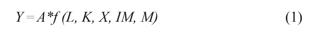
where Y, A, L, K, X, IM and M represent total production, technology, labour, capital, export, import and monetary policy indicators, respectively.

Therefore, and in line with the Esfahani (1991) approach, we consider that equation (1) is a type of a Cobb-Douglas production function which exhibits constant returns to scale:

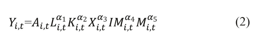
where α_i is a parameter lying between 0 and 1, representing the elasticity of the product with respect to labour (α₁), capital (α₂), export (α₃), import (α₄), and monetary policy indicators (α₅) for country i during the time period t.

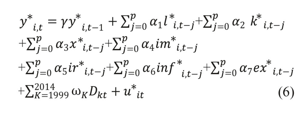
Taking the translog forms from both sides of equation (2), the final version of the production function for wine could be presented by:

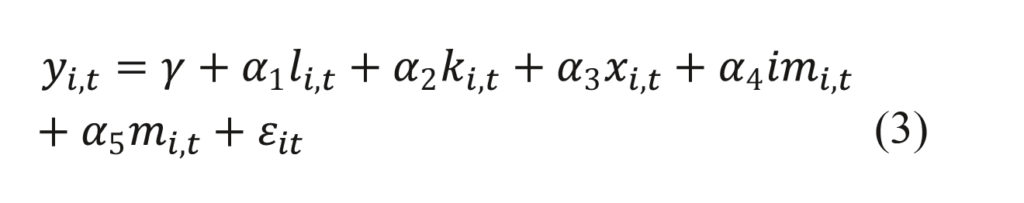
In equation 3, all the variables are lowercase because they are expressed in logarithms for country i in the year t. The variable y_i,t corresponds to the wine production, expressed by the value added at the factor cost in million euros. The five explanatory variables are the total number of persons employed in wine manufacture (l_i,t), the gross investment in the wine manufacture in million euros (k_i,t), the total value of wine exports in million euros (x_i,t), the total value of wine imports in million euros (im_i,t) and a dataset of monetary policy indicators (m_i,t). This dataset includes the real short-term interest rate, corresponding to the nominal day-to-day money market interest rate minus the inflation rate, the inflation rate, measured by the total consumer price index, and alternatively, by the producer index in industrial activities, and the real effective exchange rate, which is the weighted average of a country’s national currency relative to a basket of major currencies.

The variables are expressed in annual frequency, and they are converted into constant 2010 prices using the Consumer Price Index (CPI 2010 = 100). The data are obtained from the Eurostat, the Food and Agriculture Organisation of the United Nations (FAO) and the Organisation for Economic Co-operation and Development (OECD). Table A.1 and Table A.2 in the Appendix contain all the variables’ definitions and sources, and summary statistics of data in panel format (for the level of the variables), respectively.

3.2. Methods

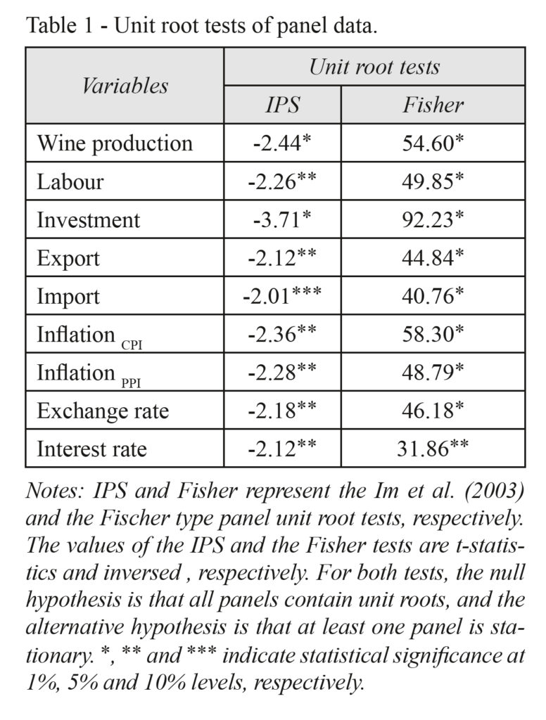
Before proceeding to the econometric estimations, and because the presence of level stationarity is an important condition for applying panel regression methods, we tested the stationary properties of the variables, applying the Im et al. (2003) and the Fisher type panel unit root tests (Table 1). The results from both tests reveal that all the series are stationary at their levels.

To estimate the regressions, we apply the dynamic panel data generalised method of moment (GMM) approach, as the explanatory variables are not strictly exogenous. Following Bond’s (2002) suggestion, we first estimate the pooled OLS and the FE models for robustness checks by means to obtain an accurate dynamic panel data GMM estimation. The following model will be estimated by using the pooled OLS:

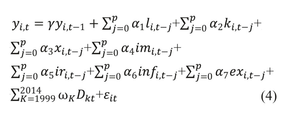
where ir, inf and ex represent the interest rate, the inflation rate and the exchange rate, respectively, and D_kt denotes the annual dummies that capture the business cycles and annual specific shocks, taking the value 1 when k = t, and 0 otherwise. The FE model is formulated as:

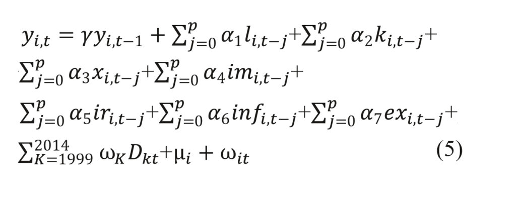
where μ_i denotes the unobserved (non-time series) country-specific effect.

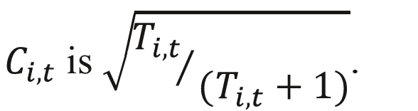
In the dynamic panel data GMM approach, we apply the forward orthogonal deviation transformation proposed by Arellano and Bover (1995). In this method, the data loss is minimised by subtracting the average of all future available variable observations rather than subtracting the previous observation from the current one. Suppose that we want to transform the y variable, the forward orthogonal transformation proceeding according to: 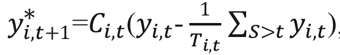where the sum is taken over available future observations, T_i,t is the number of such observations, and the scale factor is

One property of this transformation is that if y_i,t are independently distributed before transformation, they remain so afterwards. The model using data with this type of transformation is expressed by:

The dynamic panel data GMM method is designed for situations with a linear functional relationship, where the dependent variable depends on its own lagged values, the independent variables are not strictly exogenous, and there are fixed individual effects, heteroscedasticity and autocorrelation within the errors of individual units.

4. Results and discussion

The results obtained from the one-step forward orthogonal deviation-GMM are unbiased according to Bond (2002) and are reported in Tables 2 and 3. In both tables, the Hausman test represents the Hausman (1978) specification test, which chooses the FE model rather than the random effect model. The Sargan J test represents the Sargan (1958) test of over-identifying restrictions, which has indicated that the restrictions are not over-identified. The Arellano-Bond test represents the Arellano and Bond (1991) serial correlation test, which has rejected the presence of serial correlation for the three estimators. Finally, the heteroscedasticity test implemented by Breusch and Pagan (1979) and Cook and Weisberg (1983) has failed to reject the homoscedastic variances for all cases.

4.1. Results

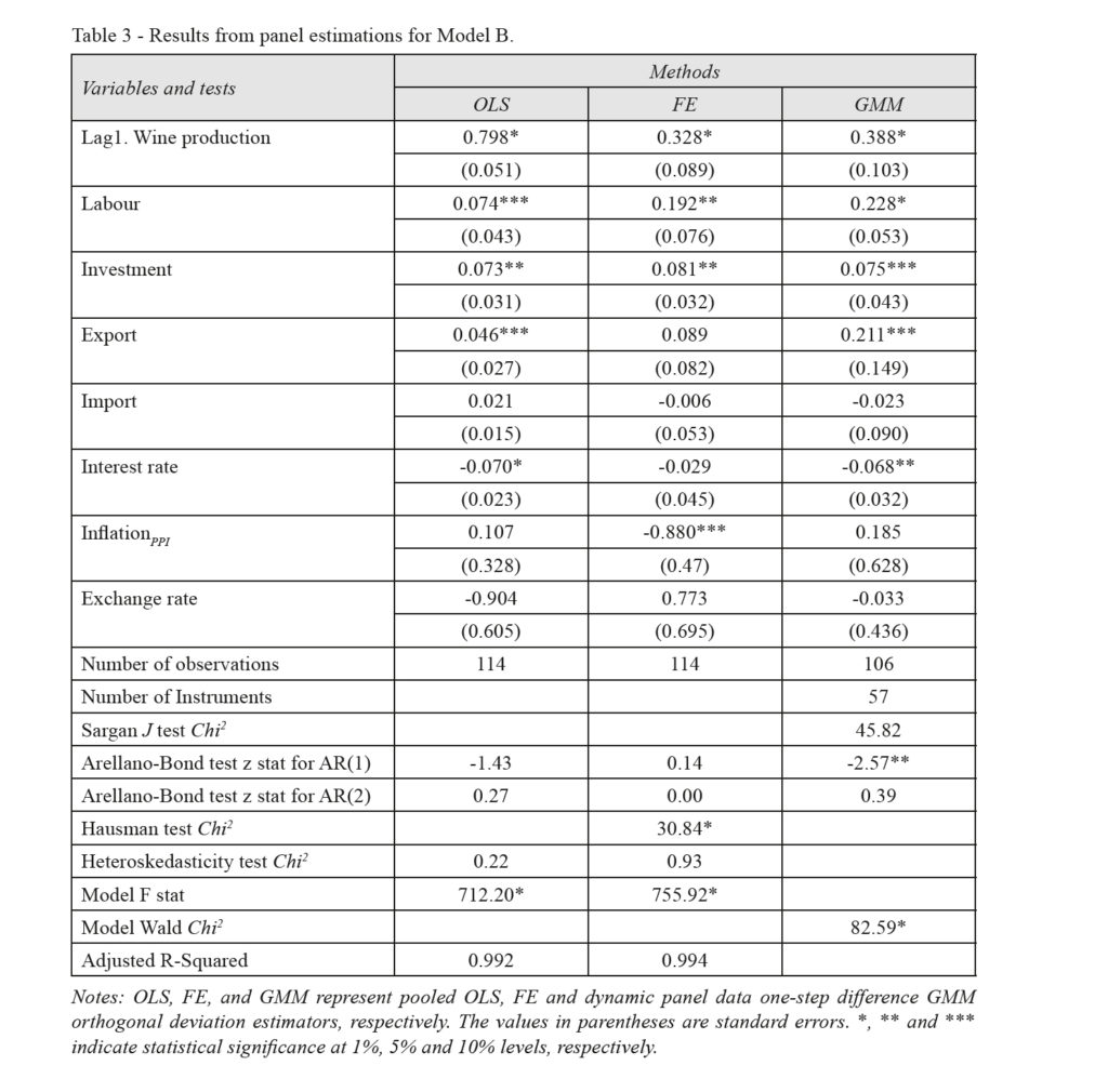
We describe the results in two subsections: Model A (Table 2) and Model B (Table 3), in which the only difference is their inflation measurement: In Model A, inflation rate is measured by the consumer price index and in Model B by the industrial producer price index.

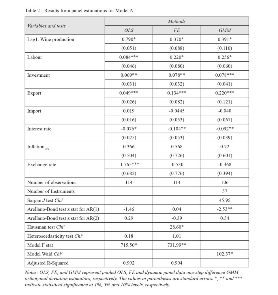
a) Model A

Regarding the impact of labour, OLS (α₁ = 0.08, P < 0.1), FE (α₁ = 0.22, P < 0.00) and GMM (α₁ = 0.26, P < 0.00) find a positive and significant effect. According to the GMM, a 1 percent increase in the number of workers leads to a 0.26 percent increase in wine production. For investment also, OLS (α₂ = 0.07, P < 0.05), FE (α₂ = 0.08, P < 0.05) and GMM (α₂ = 0.08, P < 0.1) find a positive effect. This shows that a 1 percent increase in investment leads to approximately a 0.08 percent increase in wine production, which is a very small impact.

Looking at the impact of wine exports, OLS (α₃ = 0.05, P < 0.1), FE (α₃ = 0.13, P < 0.1) and GMM (α₃ = 0.22, P < 0.1) find evidence for a positive association between exports and wine production. According to GMM, a 1 percent increase in export leads to a 0.22 percent increase in wine production. Concerning the effect of wine imports, none of the estimators shows an impact from this factor.

Looking at the impact of the interest rate, OLS (α₅ = -0.08, P < 0.00), FE (α₅ = -0.10, P < 0.05) and GMM (α₅ = -0.09, P < 0.05) find a negative association between the interest rate and wine production. This means that a 1 percent increase in the interest rate causes wine production to decrease about 0.1 percent. Regarding the impact of the exchange rate, only OLS (α₇ = -1.76, P < 0.00) finds evidence for a negative impact of the real effective exchange rate on wine production. Finally, none of the estimators indicate an impact of the consumer price index on wine production.

b) Model B

The results for Model B are qualitatively similar to those obtained from Model A, with small differences in the magnitude of the estimators, for the impact of labour, investment, exports and the interest rate on wine production. Moreover, in the case of wine imports, there is a consistent result of no significant impact on wine production.

A comparison between Models A and B only reveals quite distinct findings concerning the effects of inflation and of the effective exchange rate. In Model B, the FE (α₇ = -0.88, P < 0.1) finds weak evidence in favour of a negative impact of PPI on wine production, but none of the estimators indicate an impact of the real effective exchange rate on wine production.

The robustness checks also confirmed the consistency of the results from the different estimators. Namely, we checked for the impact of manufacturing and food manufacturing producer price indices, and the results stayed almost robust. Additionally, we tested the inclusion of annual dummies to capture the impact of the Common Market Organisation reform in April 2008. The annual dummies results demonstrated that there is not a substantial difference between the years before and after 2008. This indicates that this reform did not significantly affect EU wine production yet.

4.2. Discussion

Our study showed that the number of persons employed and the investment in the wine sector have a positive influence on wine production. This confirms the theoretical background that exists for the wine production function, which consensually agrees that the size of manufacturing, including a higher number of workers and more investment, increases EU wine production.

Second, our results revealed that higher values of wine exports lead to a boost in wine production, while wine imports cause no effect. This result is in line with the findings of Vlacho (2017), who found a positive association between exports and wine production, but no impact from imports of wine, among European wine producers. In addition, from a broader perspective, it is in line with a vast number of studies that show the stimulating impact of higher exports on aggregate production (e.g., Marin, 1992; Ramos, 2001; Cuaresma and Wörz, 2005; Siliverstovs and Herzer, 2006; Parida and Sahoo, 2007; Shafiullah et al., 2017). Regarding policy recommendations, the findings suggest that the EU should be receptive to the implementation of free trade agreements (FTAs), as they play a strategic role in boosting bilateral trade between members. FTAs are the main resource in reducing or eliminating tariff and non-tariff barriers, and some studies (e.g. Baier and Bergstrand, 2009) even show a doubling of trade between signatory countries as a result of FTAs.

Third, as seen in section 2, there is a consensus in the literature about the negative impact on production of higher interest rates and appreciation of exchange rates. However, the effect of the inflation rate on production remains inconclusive. We did not obtain strong and consistent evidence for the impact of inflation and exchange rates but we found a solid negative effect from the short-term real interest rate on wine production. Hence, we predict that EU wine production decreases when a contractionary monetary policy is adopted. This result is in line with the European Commission (2009a; 2009b), which concluded that increases in real interest rates have a robust negative impact on manufacturing output growth in Europe.

Overall, concerning the influence of monetary indicators, our results highlight the interdependence between nominal and real economic activities. This suggests that more efficient and healthy financial markets, which affect the transmission of monetary policy, will enhance the productive sectors, implying that some efforts aimed at developing financial markets should be taken.

5. Conclusion

In this study, we evaluated the impact of several macroeconomic factors on EU wine production, with particular emphasis on monetary indicators. For this purpose, and based on the theoretical background, we have developed an extended Cobb-Douglas production function that was estimated by applying the dynamic panel GMM approach to annual data from 1999 to 2014.

In line with the results of previous studies, we have found a positive impact of labour, investment and exports on wine production. Concerning the effect of monetary indicators, we have concluded that the short-term interest rate impacts negatively on wine production. For the other two monetary variables – the inflation rate and the exchange rate – the results are not robust, and vary depending on the inflation measure used (CPI or PPI).

Our results indicate that EU wine production may be influenced by instruments of monetary policy. In particular, an expansionary monetary policy, lowering the short-term interest rate, is a useful instrument for promoting the EU wine sector. On the other hand, EU countries, specifically the ones where the wine sector plays an important role in their economic growth and has a higher share of GDP, need to be more cautious about their wine sector when the EU is adopting a contractionary monetary policy.

Our study has some limitations, mainly concerning data availability. Further research will imply an enlargement of the size of the sample and the inclusion of new explanatory variables to obtain more solid results. In particular, the inclusion of some variables of control to capture the impact of climate changes might be an accurate extension to the model in the sense that climate changes could have implications in the economic policies and, therefore, in the European wine sector.

As a final remark, we point out that this study opens the way to other interesting related research topics. A potential extension might be to analyse the fluctuations of wine production in EU member states and whether they are synchronised with European business cycles. Another issue that may be of particular interest is to explore the impact in EU wine production resulting from the entry of ‘new world’ producers, which constitutes an important challenge to the ‘old world’ regions as the production from the former has added significantly the wine available in the world market.

Acknowledgments

This work is supported by the project NORTE -01-0145-FEDER-000038 (INNOVINE & WINE
– Innovation Platform of Vine & Wine) and national funds, through the FCT – Portuguese Foundation for Science and Technology under the project UID/SOC/04011/2019.

References

• Anderson K., Nelgen S., Pinilla V., 2017. Global wine markets, 1835 to 2016: a statistical compendium. Adelaide: University of Adelaide Press.
• Arellano M., Bond S., 1991. Some tests of specification for panel data: Monte Carlo evidence and an application to employment equations. Review of Economic Studies, 58(2): 277-97.
• Arellano M., Bover O., 1995. Another look at the instrumental variables estimation of error components models. Journal of Econometrics, 68(1): 29-51.
• Baier S., Bergstrand J., 2009. Estimating the effects of free trade agreements on international trade flows using matching econometrics. Journal of International Economics, 77: 63-76.
• Bedek Ž., Njavro M., 2015. Strategic Risk Management in the Croatian wine industry upon EU accession. New Medit, 14(1): 53-60.
• Bond S., 2002. Dynamic panel data models: a guide to micro data methods and practice. Institute for Fiscal Studies, Working Paper 09/02.
• Bonfiglio A., 2006. Efficiency and productivity changes of the Italian agrifood cooperatives: a Malmquist index analysis, Università Politecnica delle Marche, Working Paper n. 250.
• Breusch T.S., Pagan A.R., 1979. A simple test for heteroscedasticity and random coefficient variation. Econometrica, 47(5): 1287-1294.
• Castillo J., Villanueva E., García-Cortijo M., 2016. The international wine trade and its new export dynamics (1988-2012): a gravity model approach. Agribusiness, 32(4): 466-481.
• Conradie B., Cookson G., Thirtle C., 2006. Efficiency and farm size in Western Cape grape production: pooling small datasets. South African Journal of Economics, 74(2): 334-343.
• Cook R.D., Weisberg S., 1983. Diagnostics for heteroscedasticity in regression. Biometrika, 70(1): 1-10.
• Cuaresma J.C., Wörz J., 2005. On export composition and growth. Review of World Economics, 141(1): 33-49.
• Di Nino V., Eichengreen B., Sbracia M., 2011. Real exchange rates, trade, and growth: Italy 1861-2011, Banca d’Italia, Economic History Working Paper 10.
• Durlauf S., Kourtellos A., Tan C.M., 2008. Are any growth theories robust? The Economic Journal, 118(527): 329-346.
• Esfahani H.S., 1991. Exports, imports, and economic growth in semi industrialized countries. Journal of Development Economics, 35(1): 93-116.
• European Commission, 2009a. European competitiveness report 2008. Luxembourg: European Commission.
• European Commission, 2009b. Sectoral growth drivers and competitiveness in the European Union. Luxembourg: European Commission.
• Fischer S., 1993. The role of macroeconomic factors in growth. Journal of Monetary Economics, 32(3): 485-512.
• Gergaud O., Ginsburgh V., 2010. Natural endowments, production technologies and the quality of wines in Bordeaux. Does terroir matter? Journal of Wine Economics, 5(1): 3-21.
• Giuliani E., Morrisson A., Rabellotti R., 2011. Innovation and technological catch-up in the wine industry: an introduction. In: Giuliani E., Morrisson A., Rabellotti R. (eds.), Innovation and technological catch-up: The changing geography of wine production. Cheltenham: Edward Elgar.
• Glüzmann P.A., Levy-Yeyati E., Sturzenegger F., 2012. Exchange rate undervaluation and economic growth: Díaz Alejandro (1965) revisited. Economics Letters, 117(3): 666-672.
• Goodhue R.E., LaFrance J.T., Simon L.K., 2009. Wine taxes, production, aging and quality. Journal of Wine Economics, 4(1): 27-45.
• Hausman J.A., 1978. Specification tests in econometrics. Econometrica, 46(6): 1251-1271.
• Henriques P.D.S., Carvalho M.L.S., Costa F., Pereira R., Godinho M.L.F., 2009. Characterization and technical efficiency of Portuguese wine farms. Ciência e Técnica Vitivinícola, 24(2): 73-80.
• Im K.S., Pesaran M.H., Shin Y., 2003. Testing for unit roots in heterogeneous panels. Journal of Econometrics, 115(1): 53-74.
• International Organization of Vine and Wine, OIV, 2017. State of the vitiviniculture world market, http://www.oiv.int/public/medias/5287/oiv-noteconjmars2017-en.pdf.
• Ireland P.N., 2008. Monetary transmission mechanism. In: Durlauf S.N., Lawrence E., Blume L.E. (eds.), The new Palgrave dictionary of economics, 2^nd ed. Houndmills (UK): Palgrave MacMillan.
• Kormendi R.C., Meguire P.G., 1985. Macroeconomic determinants of growth: cross-country evidence. Journal of Monetary Economics, 16(2): 141-163.
• Marin D., 1992. Is the export-led growth hypothesis valid for industrialized countries? The Review of Economics and Statistics, 77(4): 678-688.
• Moreira V.H., Troncoso J.L., Bravo-Ureta B.E., 2011. Technical efficiency for a sample of Chilean wine grape producers: a stochastic production frontier analysis. Ciencia e Investigación Agraria, 38(3): 321-329.
• Parida P., Sahoo P., 2007. Export-led growth in south Asia: a panel cointegration analysis. International Economic Journal, 21(2): 155-175.
• Ramos F.F.R., 2001. Exports, imports, and economic growth in Portugal: evidence from causality and cointegration analysis. Economic Modelling, 18(4): 613-623.
• Rodrik D., 2008. The real exchange rate and economic growth. Brookings Papers on Economic Activity, 365-412.
• Sargan J., 1958. The estimation of economic relationships using instrumental variables. Econometrica, 26(3): 393-415.
• Sellers-Rubio R., Sottini V.A., Menghini S., 2016. Productivity growth in the winery sector: evidence from Italy and Spain. International Journal of Wine Business Research, 28(1): 59-75.
• Shafiullah M., Selvanathan S., Naranpanawa A., 2017. The role of export composition in export-led growth in Australia and its regions. Economic Analysis and Policy, 53: 62-76.
• Siliverstovs B., Herzer D., 2006. Export-led growth hypothesis: evidence for Chile. Applied Economics Letters, 13(5): 319-324.
• Tóth J., Gál P., 2014. Is the new wine world more efficient? Factors influencing technical efficiency of wine production. Studies in Agricultural Economics, 116(2): 95-99.
• Vlachos V.A., 2017. A macroeconomic estimation of wine production in Greece. Wine Economics and Policy, 6(1): 3-13.
• World Trade Organization, 2004. International trade and macroeconomic policy, World Trade Report, https://www.wto.org/english/res_e/booksp_e/anrep_e/wtr04_2a_e.pdf.

Appendix